Theoretical cases for validation

One of the steps in responsible design process is validation. To validate a design it is often good to use simple reliable theoretical cases to measure against. The following are such cases.

These cases describe the equations and assumptions used in achieving the validation of a simulation output.

Displacement, the Mass-Spring Case

A simple mass and spring validation case.

Newton’s law:

(1)

With:

	Numerical value:
: position, based on time t
: velocity
: acceleration
= mass of the body in kg	10
= spring damping in N.s/m	20
= spring stiffness in N/m	15000
= spring free length in m	0.3
= gravity in m/s2	9.81
initial position in m	0.33
= initial velocity in m/s	0.0

(1)
with
	(2)
A solution for this differential equation is:
	(3)
A particular solution, when the system is stabilized, is for and x = B.
Then (2)
	(4)
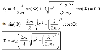
The initial conditions give the value of A and :
for t = 0.0, (3)
	(5)
	and
	(6)
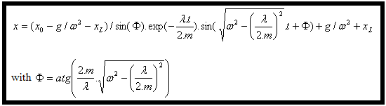
Finally, (4) and (6) reported in (3) gives the equation of the displacement :
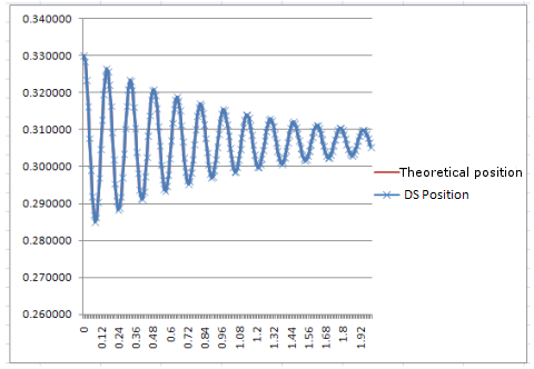
This equation was then programmed in Excel and the results compared with the results produced by Dynamic Simulation, the results being identical.

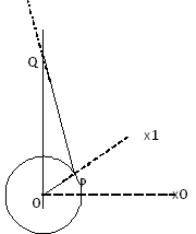
Position and Velocity, the Crank-Piston Case

The purpose of this validation case is to check the position and velocity in a crankshaft and piston mechanism when output from dynamic simulation in comparison with theoretical equations describing the same.

Known values: The “throw” or distance of the crankshaft journal from the rotational center of the crankshaft, and the length of the connecting rod between the main bearing journal and the piston pin joint.

Diagram

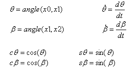
Definition	R = length(OP) = crankshaft throw L = length(PQ) = connecting rod length
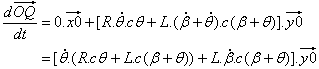
Velocity of point Q in relation to the absolute coordinate system R0 = (x0, y0)
	// position of Q in R0
	//velocity of Q in R0
with:
and:
with:
and;
then:
Point Q stays on the y0 axis and the x0 component is 0.0 :
Finally, using (1):
Equation (1) gives : which is not linear based on time; so then is not a constant and is not a simple periodic function.
(1)
and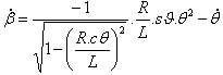
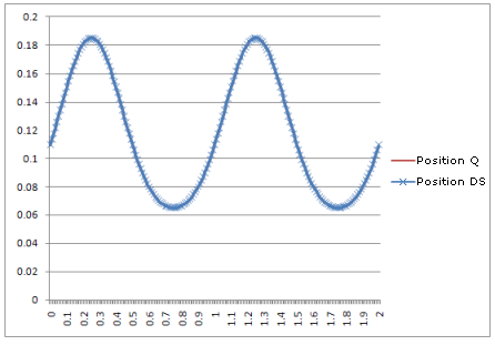
Using MS Excel and numerical values (L=0.125m, R=0.06m, and rad/s), we compute the position and the velocity of point Q as follows:
Position:
Velocity:

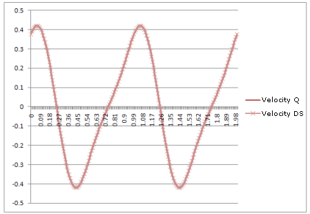The result: curves in dynamic simulation are identical to the curves produced by the theoretical equations.