Select a curve

When using the Input Grapher to define values that vary over the simulation , you have various options for defining curve sectors. These options are in the form of laws or mathematical functions that create specific curve types.

Note: When outputs are consumed in a user-defined formula, their browser name is appended with the output owners name in parentheses. For example: “Force (Revolution:7)”

Select mathematical functions and define their parameters

To define each sector of a curve, assign mathematical functions (that is, laws). You can create several successive sectors that each has its own law or a sum of different laws, for instance, a sine function plus a ramp function. You can, for example, create a first sector with a cubic ramp and a second sector with a sine. The software imposes the continuity principle of the global laws. This behavior can confuse the second sector's first point and the first sector's last point and cause other points to move automatically. Often, to get the curve you initially wanted, you must add additional functions.

After you select a law and move it to the List of sector's laws box, add parameters for the law. To add parameters you must do the following:

After you select a curve sector and add any conditions you want to apply, you are ready to define the selected curve sector.

In the List of available laws box, click the down arrow and select the law you want to use.
Click to replace the sector's current law with the one selected in the sector list.
You can select and replace laws as often as you like, but the new law overwrites the law displayed in the List of sector's laws box.

You can sum multiple laws on the same sector. If you want to add additional laws for a sector, repeat the first step and this step, but click instead. To remove a law on a sector that contains multiple laws, select the unwanted law in the List of sector's laws box and click .

Enter the necessary properties for the law displayed in the List of sector's laws box.

If you display

Enter

Linear ramp, Cubic ramp, Cycloid, Harmonic, Modified sine, Modified trapezoid

The coordinates (X1, Y1) and (X2, Y2) of the points that define the curve and/or enter a value for Slope to set the average gradient of the line. The curve can be defined either by entering the coordinates of the start and endpoints or by entering the coordinates of the start point and the average gradient of the sector.

The curve is symmetrical about the middle of the sector.

The area under the curve is equal to the area of the triangle beneath an equivalent linear ramp.

Linear ramp has a constant slope, that is, the two points of the sector are linked by a straight line.

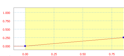
Linear ramp with a slope of 30 in/s.

Cubic ramp is defined by a 3rd order polynomial.

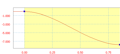
Cubic ramp with an average slope of 70 in/s.

Cycloid is a ramp function from sine/cosine.

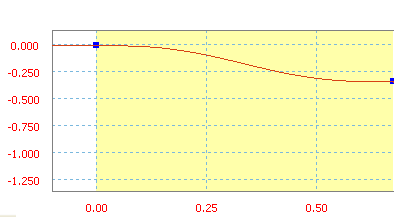
Cycloid ramp with an average slope of -50 in/s.

Harmonic is a ramp function from sine/cosine.

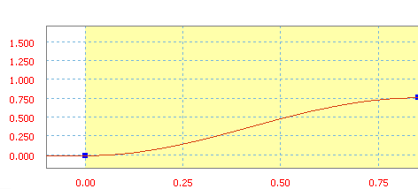
Harmonic ramp with an average slope of 90 in/s.

Modified sine is a ramp function from sine/cosine.

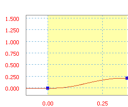
Modified sine ramp with an average slope of 60 in/s.

Modified trapezoid is a ramp function from sine/cosine.

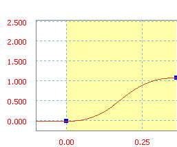
Modified trapezoid ramp with an average slope of 300 in/s.

If you display	enter
Sine	a value for Amplitude to show the height of the curve from the cycle median, for Frequency to show the number of cycles per X axis unit, and for Phase to show the distance from the start of a cycle to the start of the sector. Sine is a classical function. The units of the amplitude are the same as for the controlled variable (imposed motion, force). The units for the frequency are the inverse of the variable used for the X axis (in Hz if it is time). The phase is in degrees or radians.
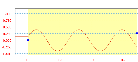
Sine with an amplitude of 40, a frequency of 3 Hz, and a phase of 20 degrees.
Polynomial	Polynomial is a polynomial function and, in this case, it has up to five degrees. There are two methods for defining the coefficients for the polynomial. Method 1 - Specify the coefficient values Enter a value for a0 and as many of the next a values as you wish. Method 2 - Import a text file opens the Open dialog box, enabling you to import a file that defines this polynomial. Order sets the order of the polynomial for the curve in the selected sector. calculates the constant value and the values at the first five orders of this polynomial. a0, a1, a2, a3, a4, a5 shows the constant value and the values at the first five orders of this polynomial. You can edit these values if necessary. The text file should be formatted as follows: //comments - comment lines are optional and are preceded by two slashes. x1 y1 - list of points using x and y values. ... - one point definition per row or line. xn yn - as many points as you require. You can enter the appropriate values or the software can automatically calculate the terms by using the least squared interpolation method.
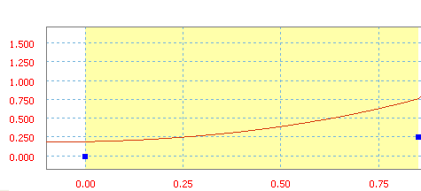
Polynomial with a0=20 in, a1=10 in/s, a2=50 in/s², and a3=20 in/s³.
Spline	A value for Slope to set the slope of the line. Spline is a cubic function used to interpolate between successive points. There are several ways you can define a spline. They are: You can quickly define the input points with the mouse in the graph region by double-clicking or by right-clicking and selecting Add Point. However, the software treats this sector as a succession of sectors instead of a single curve sector. You can enter more precise coordinates by importing a text file. Initial slope sets the slope of the first point. Final slope sets the slope of the final point. You can load a previously defined spline.
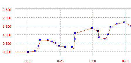
Spline defined by adding points.
You can save the spline you define here, regardless of how you defined it. Note: You cannot add other laws to a sector defined by a spline. Also, if you replace a sector's law by a spline, then the initial and final slopes are automatically collected from the previous and following sectors, but can be manually modified later.
If you want to use a text file containing tangency points, structure the file as follows:
// comments	You may include one or more lines of commentary in the file. Each line must start with “//”. Comment lines are optional, but provide value by enabling you to note the purpose of the spline.
[Tangents] T1 T2	Specify the value of the tangent for the beginning (T1) and ending (T2) points of the sector. These values are shown as the “initial” and “final” slope in the user interface. If no value is supplied, an implied tangent value of 0.0 (horizontal tangent) is assumed. As with comment lines, this line is optional, but as noted, where no tangent value is given some assumptions must be made.
X₁ Y₁ ... X_n Y_n	The list of point coordinates, you can list as many points as you need. Define one point per row.
Example text file	// // Simulation input spline points // Value: Joint Torque (N mm) // Reference: Time s [Tangents] -3.40775 -5.27803 +0.000 +0.000 +4.313 +1.510 +7.954 -9.756 +1.000 +0.000
Formula	a formula in the formula box to define the curve. Formula is an equation with functions and keywords. Available only for the definition of the joint and external efforts. You cannot impose a motion on a degree of freedom. Continuity with the adjoining sectors is not automatically maintained. Define them to avoid collision during the simulation. Formulas are limited to 255 characters. You can use any of these functions: abs fmod a cos cos log10 sqrt asin sinh log sqr atan sin pow trunk atan2 tanh sign pow10 floor cosh tan sign0 exp round
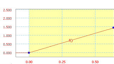
Curve defined by the formula Y = X + 37,

Example 1

You create three sectors. In the second, you want a low frequency sine.

You see the curve before and after the sine's creation. The third sector has moved vertically for the continuity between the two sectors. To get the curve you initially wanted, you must add additional functions.

Example 2

Some functions are limited in their definitions. To get a sine varying around 300, you have to add a constant law of value 300 and a sine law.

Note: The order of the law's addition is not important.

Variation around a non-nil slope can be modeled by the combination of a ramp and a sine.

Example 3

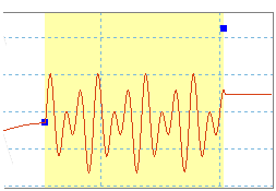
To simulate a vibration in an alternative motion, combine sine laws of different amplitudes and frequencies.

Define values outside a curve sector

It is interesting to define how the variable behaves outside of the curve sectors: before the first and after the last. After you select an area outside the entire curve and add any conditions you want to apply, you are ready to define the selected area.

Select a definition for the selected area outside a curve.
If you select Cyclical, click Start.
The Selection of a starting point dialog box opens.
On the Selection of a starting point dialog box, click the down arrow on the right of the field.
A menu opens and shows every point that begins a curve sector.
Click the point beginning the curve sector you want to copy for this area.
Click OK.

You have five choices for a definition of the area outside a curve. They are:

Constant value	This setting sets a constant value equal to either the first value in the curve if you are defining the area on the left of the first point or the last value in the curve if you are defining the area on the right of the last point. This setting is the default.
Constant slope	This setting defines a line of constant slope in the selected area. The value of the slope is equal to either the value of the slope for the first curve sector if you are defining the area on the left of the first point or the value of the slope for the last curve sector if you are defining the area on the right of the last point.
Modulo	This setting defines a value in the definition range of the law (all sectors being defined) according to the modulo principle, that is, a curve that is defined is repeated on both sides of the ordinate axis. Dynamic Simulation checks that the ordinate of the last point of the law (last sector) is equal to the ordinate of the first point (first sector). If not, you see an error message instructing you to modify the values. This message appears because the computation engine cannot handle discontinuities. This mode is applied on the right and left-hand parts of the law.
Cyclical	This function uses a cycle copied from a user-defined point until the last point in the user-defined curve. For the start of the cycle, select a point that is equal to the last point in the user-defined curve. Otherwise there is a discontinuity between the start and end of the cycle. In this case, you see an error message.
Free	This setting sets no definition for this area. No force is applied and the degree of freedom that is driven (with an imposed motion) becomes free. For an imposed motion, it is necessary to free the right-hand sector of the last point before freeing the last sector, then the sector before the last, and so on.