A large pressure drop is often observed when the melt passes through contractions in the feed system, such as between the sprue, runners and gates, at the entrance of the die. Typically 85% of the pressure loss occurs at the entrance of the die, and 15% at the exit.
Shear viscosity, fluid inertia and extension viscosity also contribute to this juncture loss. The juncture loss model is derived from flow experiments to characterize the pressure drop. The juncture loss model can be used to improve the predictions of pressure and flow balance in the feed system.
The juncture loss model relates the entrance pressure drop,  , to the wall shear stress,
 , at the contraction.

 is measured pressure loss,
- is the pressure loss at the entrance junction,
 is the pressure loss through the die, and
  is the pressure loss at the exit junction.
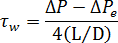
 is the length and
 is the diameter of the entrance junction.
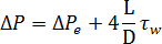
When plotting capillary  vs. measured pressure drop, the intercept at
  would be the extra pressure loss and the slope would correspond to
  .
.
It was found experimentally that the results of the extra pressure losses at various temperatures and shear rates can be collapsed onto a single master curve (for a given generic grade of material), by plotting the extra pressure loss versus the wall shear stress.
The following correlation, originally developed by Munstedt, is used to relate the extra pressure loss to the wall shear stress in the capillary data analysis. 1
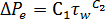
 and
and  , are derived from a series of capillary viscosity experiments with different die lengths. Measurements using different capillary die sizes are made to correct for the juncture losses. The overall pressure drop for each experimental run is simulated using the finite difference simulation and an optimization procedure is used to iterate upon all the WLF model constants as well as the and constants until the RMS deviation between the predicted and the measured pressure drop is minimized.
 A better approach might be to note the range of the coefficients and typical values.
There is a relationship between the coefficients, so as increases, decreases.
= 1e-5 to 10 (typically 0.0001)
= 2.5 to 1 (typically 2)
If juncture loss data is not available for the material that you selected, you can evaluate whether juncture loss is significant to your application by running Fill analyses with and without juncture loss coefficients. For this purpose, you can use typical values for the juncture loss coefficients, and enter these into the material data. There is an inverse relationship between the coefficients, so as increases, decreases. values range from 0.00001 to 10 (typically 0.0001), while values range from 2.5 to 1 (typically 2). If analysis results show that juncture loss is significant to your application, it is strongly recommended that you have the material characterized by Autodesk Moldflow Plastics Labs for juncture loss coefficients.