Result viewing techniques

In this task you will practice some result viewing techniques.

In this task, you will:

• View and synchronize multiple results.
• Synchronize different studies.
• Overlay results.

The tutorial model is shown in the image below: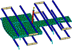

The Split tools allow you to divide the active pane into smaller panes. This is useful for viewing results on different sections of the part geometry or different results simultaneously. Select from Split, Split Vertically, or Split Horizontally.

The Locking tools are used in conjunction with split panes and allow you to coordinate the manipulation of more than one model view at the same time. Select from Lock View, Lock Plot, and Lock Animation.

1. Click (Get Started tab > Launch panel > New Project).
2. Enter Postprocessing in the Project name text box.
3. Click OK.
4. Click (Home tab > Import panel > Import).
5. Navigate to the Tutorial folder, typically C:\Program Files\Autodesk\Simulation Moldflow Insight 20xx\tutorial, where xxxx is the software version.
6. In the Files of Type drop-down list, select Study Files (*.sdy).
7. Select cpu_base.sdy and then click Open.
8. Click (View tab > Navigate panel > Orbit) and rotate the model to examine its geometry and features. Notice in the Study Tasks pane that the tutorial model is represented by a Dual Domain Mesh. It contains one injection location and four cooling circuits.
9. Select Fill time from the Results section of the Study Tasks pane.
   Tip: To display a result, select the check box next to the result name in the Study Tasks pane.
10. Click Split Horizontally. The screen is split and a duplicate of the model is displayed in the lower portion of the screen.
    The split pane tools work as a toggle. Use them to turn the splits on and off. Turning a split off removes any specific formatting settings for that pane.

    Note: The dotted line inside the upper pane indicates that this is the active pane.
11. Click inside the lower pane. This is now the active pane.
12. Select Pressure at end of fill from the Results section of the Study Tasks pane.
    Note: The analysis result type is displayed in the upper right corner of each model pane.
13. Rotate and zoom in on a section of the model and note how the image in the upper pane has not altered. This allows you to view different results in different parts of the model.
    
    
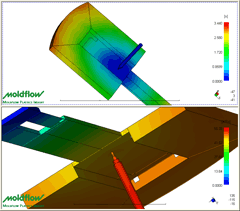
14. With the bottom pane still active, select Fill time from the Results section of the Study Tasks pane. This allows you to view the same result in different parts of the model.
15. To synchronized views, click Split Vertically. You should now have four panes showing.
16. Activate the top-left pane and select Bulk temperature at end of fill in the Results section of the Study Tasks pane.
17. Click Lock View.
18. Activate the top-right pane and select Volumetric shrinkage in the Results section of the Study Tasks pane.
19. Click Lock View from the Viewer toolbar.
20. Activate the bottom-left pane and select Circuit metal temperature from the Cool folder in the Results section of the Study Tasks pane. Ensure the Channel layer is selected in the Layers Panel for this result to display.
21. Activate the bottom-right pane and select Deflection, all effects: Deflection from the Warp folder in the Results section of the Study Tasks pane.
22. Click in the top-right pane, select (View tab > Navigate panel > Orbit) and rotate the model.

    The two top panes are locked together.

    Other model manipulation features work similarly. Experiment with:

    • (View tab > Navigate panel > Zoom All).
    • (View tab > Navigate panel > Home View).
    • (View tab > Navigate panel > Zoom Window).
    • (View tab > Navigate panel > Pan).
    • Deselect layers from the Layer Panel.

    To include the other panes in the synchronization, you could select each pane individually and then click on the Lock View icon. Alternatively, click (Results tab > Locking panel > Lock All View).

23. Activate the top-left pane and click Lock View. The icon is removed from the top-left corner of the pane. This removes the lock manipulation function. Place the mouse cursor in the top-left pane, select (View tab > Navigate panel > Orbit) and rotate the model. This is the only model that rotates.
24. You can also synchronize different studies. You will now investigate the effect that changing the injection location has on weld lines. Click on the Split pane tools and ( View tab > Windows panel) to remove the splits and display only one model.
25. Select Weld lines in the Results section of the Study Tasks pane.
26. Right-click on Part surface in the Layers panel and select Hide All Other Layers.
27. Rotate the model to -50 -25 5 by entering these values in the Rotation Angle box (View tab > Viewpoint panel > Rotation Angle).
28. Ensure the Lock View and Lock Plots icons are displayed in the top-left corner of the Model pane. If they are not present, select them from View tab > Locking panel.
29. Click (Home tab > Import panel > Import) and navigate to the Tutorial folder, typically C:\Program Files\Autodesk\Simulation Moldflow Insight 20xx\tutorial.
30. Select inject.sdy and then click Open.
31. Select Weld lines from the Results list in the Study pane.
32. Click (Results tab > Locking panel > Lock View). At the bottom of the Model pane are two tabs, one for each of the open studies. Click alternatively on these two study tabs to see the effect of changing injection locations.
33. Rotate the image and zoom in on the weld lines in the body of the model.
34. Click on the other study tab. The orientation between studies has been maintained.
35. To overlay results and combine them on one model, ensure the cpu_base model is active.
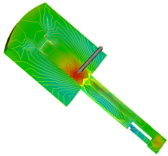
36. Select Air traps in the Results section of the Study Tasks pane. Rotate the model to find the air traps on the bottom surface of the part.
37. Right-click on Fill time in the Results section of the Study Tasks pane.
38. Select Overlay from the menu that appears.
39. Rotate the model to view the combined results.

    Results such as Volumetric shrinkage at ejection and Bulk temperature at end of fill , which are normally represented by solid shaded colors, cannot be overlayed in this manner.

40. Select Bulk temperature at end of fill . Right-click on the name in the Study Tasks pane and select Properties from the menu that appears.

    The Plot Properties dialog appears. This dialog will be discussed in a later task.

41. Select the Methods tab from the top of the dialog.
42. Select the Contour option and click OK.

    The results are displayed in contours.

43. Right-click on Volumetric shrinkage at ejection and select Overlay. Rotate the model to investigate the result.
    
    
    Note: The scale range on the right of the Model pane represents the Volumetric shrinkage at ejection result. Right-click on Bulk temperature at end of fill in the Study Task pane and select Activate to display this value range.

Click the Next topic link below to move on to the next task of the tutorial.