Thick composite elements are three- or four-node isoparametric thick plate elements formulated in three-dimensional space. These elements are based on the Mindlin theory and support the Tsai-Wu, maximum stress and maximum strain failure criteria. Core-crushing stresses can be obtained. Thick composite elements are used to model structures such as aerospace and other composite material products.
The highest surface number among the lines that define the element determines the surface number of that element. The surface number controls element loads such as pressure.
The out-of-plane rotational DOF is not considered for thick composite elements. You can apply the other rotational DOFs and all the translational DOFs as needed.
When to Use Thick Composite Elements
- To model a plate element consisting of multiple layers with one layer much thicker than the others.
- The length and width of the plate is at least 2 to 3 times the thickness.
- The elements are initially flat (planar).
Orient the Laminae in Thick Composite Elements
To clarify the terminology, a laminate is a bonded stack of laminae (layers). Each element is a laminate. The multiple laminae through the thickness are oriented at various directions relative to the laminate direction. For most element types, two sets of axes are sufficient to define the position and orientation of the element. With composite elements, four sets of axes are used.
Global Axes
The global axes X, Y and Z are the reference axes to define the coordinates at the nodal points of the finite element model.
Element Axes
Each thick composite element has its own set of local axes. See also Controlling the Orientation of Thick Composite Elements below.
Quadrilateral elements: The origin of the element axes a, b and c is defined at the centroid of the element N1-N2-N3-N4. The local a-axis is defined as going from the midpoint of side N1-N4 to the midpoint of side N2-N3. The local c-axis is defined as the vector perpendicular to the plate element using the right-hand rule with respect to node numbering (N1 -> N2 -> N3 -> N4). Refer to Figure 1.
Triangular elements: The origin of the element axes a, b and c is defined at the first node, N1, of the element N1-N2-N3. The local a-axis is defined going from node N1 to node N2. The local c-axis is defined as the vector perpendicular to the plate element using the right-hand rule with respect to node numbering (N1 -> N2 -> N3). The local b-axis is defined as the vector perpendicular to the a-axis and c-axis obeying the right-hand rule. Refer to Figure 3.
Laminate Axes
The laminate axes x, y and z are the arbitrary reference axes used to define the intersecting angle of each layer with respect to the laminate. Refer to Figure 1.
The angle α is measured counter-clockwise ( follows the right-hand rule about the local element c axis) from the positive local element a-axis to the laminate x-axis. Refer to Figure 1. This angle can be defined in the General tab of the Element Definition dialog box using the Material Axis Orientation section. If the Use Specified Angle option is selected, the laminate axis x is oriented in the element plane and at the specified angle to the element an axis. The element normal acts as laminate material axis z, and laminate material axis y is determined by the right-hand rule (z X x = y). If the Use Specified Vector option is selected, a user-defined vector is specified by the origin and the entered point. This vector is projected onto the element, and the projection acts as laminate axis x. The element normal acts as laminate axis z, and laminate axis y is determined by the right-hand rule (z X x = y). The angle α is determined by the processor in this case.
Lamina Axes
The layer 1-axis is the axis along the fiber of each individual layer. The layer 2-axis is the axis perpendicular to the fiber of each individual layer and in the plane of the element. The layer 3-axis is perpendicular to the element and therefore parallel to the local element axis c.
The layers are numbered in the positive local element c-axis. See Figures 2 and 3.
The angle ϑ is measured counter-clockwise ( follows the right-hand rule about the local element c axis) from the positive laminate x-axis to the layer 1-axis. Refer to Figure 1. This is specified in the Orientation Angle column of the Composite Laminate Stacking Sequence table in the Laminate tab of the Element Definition dialog box.
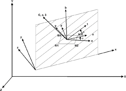
Figure 1: Example of Typical Composite Element and Definition of Composite Angles
You enter the angle α i (Use Specified Angle) or the processor calculates it (Use Specified Vector). You enter the angle ϑ for each lamina.
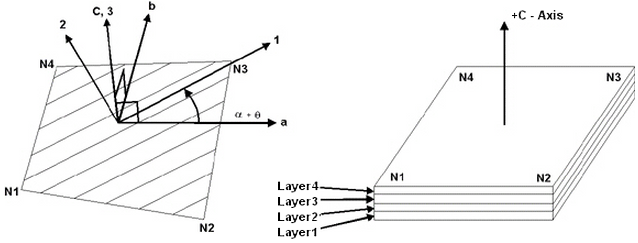
Figure 2: Example of Local Element Axes abc, Layer Axes 123 and Layer Numbering
Axis 1 is parallel to the fiber, axis 2 is in the plane of the element and perpendicular to the fiber, and axis 3 is perpendicular to the plane of the element.
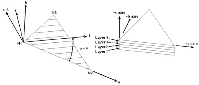
Figure 3: Example of Local Element Axes a-b-c, Layer Axes 1-2-3 and Layer Numbering for Triangular elements
You enter the angle α (Use Specified Angle) or it is calculated by the processor (Use Specified Vector). You enter the angle ϑ for each lamina.
Thick Composite Element Parameters
When using thick composite elements, you have three failure criteria available. These can be selected in the Failure Criteria drop-down menu in the General tab of the Element Definition dialog box. If the None option is selected, no failure analysis is performed. The three options are described in the following sections.
Tsai-Wu
If this option is selected, the Tsai-Wu (or quadratic tensor polynomial) criteria is used to determine if the part fails the structural analysis. This criteria, considering the interaction between stresses in two directions, for an orthotropic layer under plane stress condition, is determined by the equation:
|
|
(1) |
where
![]()
![]()
![]()
![]()
![]()
X t = Axial or longitudinal strength in tension (>0)
X c = Axial or longitudinal strength in compression (>0)
Y t = Transverse strength in tension (>0)
Y c = Transverse strength in compression (>0)
S = Shear strength
F 12 = stress interaction material property determined from biaxial tests. If F 12 is greater than 0 and these two conditions are not met, then F 12 is set equal to 0:
![]()
σ 1 = Stress in principal material 1- direction
σ 1 = Stress in principal material 2- direction
τ 12 = Shear stress in principal material 1-2 plane
The value F in equation 1 is output to the filename.s file for each layer.
Maximum Stress
If this option is selected, the maximum stress criteria is used to determine if the part fails the structural analysis. The criteria is given as:
In-plane criteria
|
|
(2) |

Out-of-plane criteria
|
σ core < Z c τ 13 < S 13 (3) τ 23 < S 23 |
σ 1 = Calculated stress in 1 direction
σ 2 = Calculated stress in 2 direction
σ core = Calculated normal stress in the core lamina (3 direction)
τ 12 = Calculated shear stress in the plane of the element (1-2 plane)
τ 13 = Calculated shear stress in the plane normal to the element (1-3 plane)
τ 23 = Calculated shear stress in the plane normal to the element (2-3 plane)
X c = Allowable compressive stress in 1 direction (>0)
Y c = Allowable compressive stress in 2 direction (>0)
X t = Allowable tensile stress in 1 direction (>0)
Y t = Allowable tensile stress in 2 direction (>0)
Z c = Allowable compressive stress of the core lamina in the 3 direction (>0)
S = Allowable shear stress in the plane of the element (1-2 plane) (>0)
S 13 = Allowable shear stress normal to the plane of the element (1-3 plane) (>0)
S 23 = Allowable shear stress normal to the plane of the element (2-3 plane) (>0)
If the three conditions of equation (2) are not satisfied, the material has failed in the in-plane direction. If the three conditions of equation (3) are not satisfied, the material has failed in the out-of-plane direction.
Maximum Strain
If this option is selected, the maximum strain criteria is used to determine if the part fails the structural analysis. The criteria is given as:
|
|
 (4)
(4) ε 1 = Calculated strain in 1 direction
ε 1 = Calculated strain in 2 direction
γ 12 = Calculated shear strain in the plane of the element (1-2 plane)
T 1c = Allowable compressive strain in 1 direction (>0)
T 2c = Allowable compressive strain in 2 direction (>0)
T 1t = Allowable tensile strain in 1 direction (>0)
T 2t = Allowable tensile strain in 2 direction (>0)
S = Allowable shear strain in the plane of the element (1-2 plane) (>0)
If the three conditions of equation (4) are not satisfied, the material has failed in the in-plane direction. No out-of-plane calculations are performed for the maximum strain failure criteria.
Specify the lamina number that defines the core of the thick composite element in the Laminate Core field. A core lamina number must always be defined. The out-of-plane shear stresses that are developed in a thick composite element are taken entirely by the one core layer specified.
The Temperature Difference for Curing is defined as T 1 -T 0 , where T 1 is the temperature at which the laminae are locked as a whole to form a laminate, and T 0 is the room temperature. The room temperature is the temperature at which the parts in the model are assembled together before the external loads (such as forces, pressures, and temperatures) are applied. (In a normal situation, the room temperature are also called the stress free reference temperature. Due to the residual stresses due to curing, the term stress free is being avoided in this discussion.) Because laminae are at various angles, the contractions of laminae of different amounts give rise to the curing stress. This curing stress is superimposed on the mechanical stresses caused by external loading.
To apply a thermal load as part of the external loading, specify the difference between the room temperature T 0 and the operating temperature T 2 in the Mean Temperature Difference field. Enter the value T 2 -T 0 . Temperatures applied to the nodes of the composite are ignored.
The Laminate tab defines the thickness of each lamina in the composite element, the orientation angle of the fiber direction (axis 1), and the material properties. You can specify the material properties for each lamina, by clicking in the Material column. See Orienting the Laminae in Thick Composite Elements above.
- To account for the mean temperature difference, the thermal multiplier needs to be assigned under the Analysis Parameters. See the page Setting Up and Performing the Analysis: Linear: Analysis Parameters: Static Stress with Linear Material Models.
- Use the Copy Row button to copy existing input to create repeating series. Either enter a single lamina to copy, or a range of lamina separated by a dash -, such as 4-8. For the Insert Before Row field, specify any row number after the last entry to insert the copy at the end of the stacking sequence.
- The Export button only saves the stacking sequence (Thickness and Orientation Angle); it does not save the material properties. Use the Save Part Attributes to File command to save this (and all the part information) to a file. See the paragraph Miscellaneous Functions (Visibility, Suppress, Copy and Paste) on the page Setting Up and Performing the Analysis: Using the FEA Editor Environment for information on the Save and Read commands.
Control Orientation of Thick Composite Elements
If the laminate axis is specified using the method Use Specified Angle, then designating which side of the element is the ij side (or N1-N2 side in Figures 1, 2, 3) is important for the proper orientation of the fibers. Recall that the lamina and laminate axes are related to the element axes which in turn are related to the ij side of the element. This is done in the Orientation tab of the Element Definition dialog box. The Method drop-down menu contains three options that can be used to specify which side of the element is the ij side. If the Default option is selected, the side of an element with the highest surface number is chosen as the ij side. If the Orient I Node option is selected, a coordinate must be defined in the X Coordinate, Y Coordinate, and Z Coordinate fields. The node on an element that is closest to this point is designated as the i node. The j node is the next node on the element following the right-hand rule about the element's normal axis (+3 axis). If the Orient IJ Side option is selected, a coordinate must be defined in the X Coordinate, Y Coordinate, and Z Coordinate fields in the Nodal Order section. The side of an element that is closest to this point is designated as the ij side. The i and j nodes are assigned so that the j node can be reached by following the right-hand rule about the element's normal axis (+3 axis) along the element from the i node.
Designating the ij side (or N1-N2 side) by itself does not control whether the node numbering N1-N2-N3-N4 is clockwise or counter-clockwise. This is controlled by specifying which direction is the positive normal direction. (The order of the layers 1, 2, 3, 4,n is also dependent on the direction of the element normal.) To do this, enter a point using the X Coordinate, Y Coordinate and Z Coordinate fields in the Element Normal section on the Orientation tab. The normal axis (axis c, z, and 3) is normal to the element and is directed away from the element normal coordinate. See Figure 4.

|
| Figure 4: Determining the Element Normal The edge-on view of the composite element is shown. |
The element normal point is also used to control the orientation of pressures applied to composite elements. A positive pressure is in the direction of the normal axis; therefore a positive pressure points away from the element normal point.
To Use Thick Composite Elements
- Be sure that a unit system is defined.
- Be sure that the model is using a structural analysis type.
- Right-click the Element Type heading for the part that you want to be thick composite elements.
- Select the Thick Composite command.
- Right-click the Element Definition heading.
- Select the Edit Element Definition command.
- To use a failure criterion in your analysis, select one in the Failure Criterion drop-down menu.
- Specify the layer that has the largest effect on the behavior in the Laminate Core field.
- If you are performing a thermal stress analysis and there is a temperature difference for curing value for your composite, enter this value in the Temperature Difference for Curing field.
- If you are performing a thermal stress analysis enter a value in the Mean Temperature Difference field. This value is the difference between the analysis temperature and the stress free temperature.
- To define the orientation of the laminate axis (x-y-z) by defining an angle, select the Use Specified Angle option in the Method drop-down menu and enter that value in the Angle field. The angle is measured counterclockwise (right-hand rule about local element c axis) from the element a axis to the laminate axes. See Figure 1.
- To define the laminate axis orientation by defining a vector, select the Use Specified Vector option in the Method drop-down menu and enter that vector in the X Coordinate, Y Coordinate and Z Coordinate fields. The angle α in Figure 1 is calculated by the processor.
- Click the Laminate tab.
- Define the thickness of each layer of the composite in the Thickness column.
- Define the lamina axis (1-2-3) for each layer relative to the laminate axis in the Orientation Angle column. This is the angle ϑ in Figure 1 above.
- Click in the Material column to specify the material properties for each layer.
- Click the Orientation tab.
- Enter an element normal coordinate. The element normal is important since the orientation angle q for each layer follows the right-hand rule about the axis normal to the element, and the direction of the layers through the thickness depends on the element normal. (Also, a positive pressure applied to the element is in the direction of the positive element normal.)
- If the laminate axis is specified using an angle (α in Figure 1), then specifying the ij side is important. Choose a Nodal Order Method and enter an appropriate X, Y, Z coordinate.
- Press the OK button.