Given:
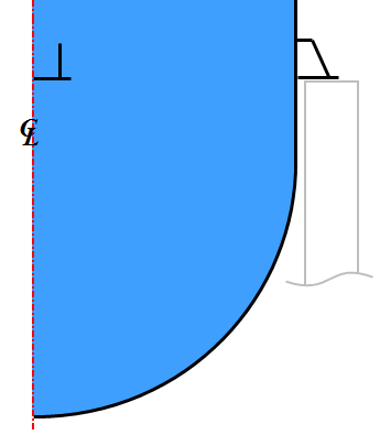
A 0.25-inch thick steel tank is supported on four base plates. The tank contains water at 150 °F and is partially filled. The tank is in a 70 °F stagnant environment.
|
Ambient air at 70°F ho = 1.5E-6 BTU/(s*°F*in 2 ) |
||
|
Heated air at 150°F hi = 4.7E-7 BTU/(s*°F*in 2 ) |
  |
|
|
Heated water at 150°F hi = 1.3E-4 BTU/(s*°F*in 2 ) |
Ambient air at 70°F ho = 1.6E-6 BTU/(s*°F*in 2 ) |
Find: The thermal stress and displacement due to the contents.
This particular analysis uses a two-step analysis procedure. First, the temperature distribution of the model is calculated using a steady state heat transfer analysis. Second, the temperature is imported into a stress analysis to calculate the thermal expansion.
This example concentrates on performing the analysis, not on the creation of the model. Therefore, the model geometry is provided. Model setup consists of applying the loads as convection, and performing the analysis.
- Start Autodesk Simulation.
- Open tank model from the Models folder of the installation directory. Use

 Archive Retrieve, browse to the Models folder, and select tank model.ach.
 - Due to symmetry, one quarter of the tank was drawn.
- The support pier is not modeled. Its effects will be included by applying boundary conditions to the model.
- The tank is drawn with +Z representing the vertical direction.
- Each portion of the tank (the tank body, support plate, and gusset) is drawn on a separate part number using plate elements. If the analysis indicates that the design is over- or under-designed, the thickness can be changed simply by changing the plate thickness (in the Element Definition).
- Different regions of the tank are on different surfaces to allow the convection loads to be applied in the heat transfer analysis, and to allow the boundary conditions and hydrostatic pressure to be applied in the stress analysis.
- The Element Type, Element Definition, and Material Properties were entered.
- The units are set to pounds, inch, second, °F, and BTU.
The effects of the hot water (and air above the water) will be simulated in the analysis by applying a convection load, as follows:
- Use surface selection Selection Shape Point or Rectangle and Selection Select Surface and click the tank body anywhere below the water level (part 2, surface 10).
- Right-click and select Add Surface Convection Load.
- Enter the Temperature Independent Convection Coefficient as 1.32E-4BTU/(s*°F*in 2 ) and the Temperature as 149 °F.
- Click OK.
- Click the tank body anywhere above the water level (part 2, surface 8).
- Right-click and select Add Surface Convection Load.
- Enter the Temperature Independent Convection Coefficient as 1.97E-6BTU/(s*°F*in 2 ) and the Temperature as 89 °F.
- Click OK.
The effects of the ambient air around the gussets will be simulated in the analysis by applying a convection load.
- Click the gusset (part 3, surface 1).
- Right-click and select Add Surface Convection Load.
- Enter the Temperature Independent Convection Coefficient as 1.6E-6BTU/(s*°F*in 2 ) and the Temperature as 70 °F.
- Activate the Apply load to both sides check box since both sides of the plate are exposed to the same condition.
- Click OK.
The effects of the heat conducting out of the support plate, into the support pier, and convecting into the environment will be simulated with a heat flux on the model, as follows.
- Click the support plate anywhere around the bolt hole (part 1, surface 7). Both plates are drawn on the same part/surface number, so both are selected by clicking on either one.
- Right-click and select Add Surface Heat Flux.
- Enter the Magnitude as -2E-4BTU/(s*in 2 ). The negative value indicates that heat is removed from the model.
- Click OK.
Use Setup Model Setup Parameters to view the Analysis Parameters dialog box. The only input required for this analysis is the Convection multiplier. This value controls the convection and heat flux. The other multipliers are acceptable with the default of 1 because there are no loads affected by the multipliers.
Run the analysis using the Analysis Analysis Run Simulation command.
Review the temperature results when the analysis is done: Results Contours Temperature Calculated Temperature. The range should be 92 to 149°F, with the following criteria:
- The tank is very uniform in temperature below the water line. The convection coefficient from the water is 100 times larger than other heat loads.
- The top of the tank cools rapidly. Although the thermal stress analysis could be performed by assuming the entire tank is at a uniform temperature, these results indicate it may not be an accurate assumption.
- The gusset and support plates do not cool down significantly even though they act like a fin.
- The temperature results are sufficiently close to the temperatures assumed for the hand calculations that another iteration is not justified at this time.
To better see the temperature drop along the top of the tank, create a path plot of the temperature.
- Change to the front view: View Navigate Orientation Front View.
- Use a rectangle to select the nodes along the edge extending into the screen: Selection Shape Rectangle, Selection Select Nodes, and draw a box just large enough to get the nodes along the top left corner.
- Right-click in the display area and choose Create Path Plot. The default plot is shown, and the Path Plot Definition dialog box is opened.
- Chances are the temperature plot looks incorrect because of the way the nodes are listed. Right-click in the Nodes list in the Path Plot Definition dialog box and select Sort By Y Coordinate. Also, choose Y Distance in the Plot Against section. The plot should be smooth.
The next stage of the analysis is to perform the stress analysis. Refer to the page Examples: Linear and Dynamic Stress: Thermal Stress of a Tank for the continuation.
Hand Calculations
One disadvantage of the plate element is that only one convection load can be applied per surface. The convection inside the tank and natural convection outside the tank cannot be applied individually. These two effects must be combined together and applied to the model as one convection load. The heat transfer on the inside and outside can be written as follows:
| Q = hi x A x (150°F - Tcalc) + ho x A x (70°F - Tcalc) |
(1) |
where h is the convection, A is the area, and Tcalc is the calculated temperature at a node. In the model, the heat transfer can be written using an equivalent convection coefficient (he) and equivalent convection temperature (Te) as follows:
|
Q = he x A x (Te - Tcalc) |
(2) |
When these two equations are set equal to each other, the unknowns he and Te can be solved by forcing the heat transferred via the calculated temperatures to be equal, and the heat transferred via the environment temperatures to be equal, or
| (hi + ho)x A x Tcalc = hex A x Tcalc |
(3) |
|
hi x A x 150°F + ho x A x 70°F = he x A x Te |
(4) |
Equation (3) yields the calculation for the equivalent convection coefficient
|
he = hi + ho |
(5) |
and solving equation (4) for the equivalent environment temperature and substituting equation (5) yields
|
Te = (150 x hi + 70 x ho) / (hi + ho) |
(6) |
The convection conditions shown in Figure 1 were calculated with the Film/Convection Coefficient Calculator, so equations (5) and (6) yield the equivalent conditions in Table 1 that are applied to the model:
Table 1: Convection Calculations
| Location |
Inside Convection hi, BTU/(s*°F*in 2 ) |
Outside Convection ho, BTU/(s*°F*in 2 ) |
Equivalent Convection he, BTU/(s*°F*in 2 ) |
Equivalent Ambient Temperature Te, °F |
|---|---|---|---|---|
| Below water level | 1.3E-4(buoyancy, turbulent vertical plate, 150 F ambient, 148 F wall, water properties at 149 F) | 1.6E-6(buoyancy, turbulent vertical plate, 70 F ambient, 148 F wall, air properties at 109 F) | 1.32E-4 | 149 |
| Air space above water level (top of tank) | 4.7E-7(buoyancy, laminar horizontal plate facing down, 150 F ambient, 105 F bulk average of top, air properties at 127 F) | 1.5E-6(buoyancy, turbulent horizontal plate facing up, 70 F ambient, 105 F bulk average of top, air properties at 88F) | 1.97E-6 | 89 |
The conduction out of the 4x8 inch support pad can be estimated by using equations for a fin. Think of the tank as sitting on a 4x8 inch concrete pier {k = 1.3E-5 BTU/(s*°F*in)}. The tank end of the pier is maintained at a hot temperature, and cooling around the pier {h = 1.6E-6 BTU/(s*°F*in 2 )} creates an arrangement identical to a fin. As an approximation, assume the pier is long enough so that the floor end is at the ambient temperature {Tamb = 70°F}. The equation for the heat loss from such as fin is
|
Q = (T-Tamb) [h x perimeter x k x A] 0.5 |
(7) |
If the pad is around 135°F, this equation yields
Q = (135-70°F) [1.6E-6 BTU/(s*°F*in 2 ) x 24 in x 1.3E-5 BTU/(s*°F*in) x 32 in 2 ] 0.5 = 8.2E-3 BTU/s
or on a per area basis, Q = (8.2E-3 BTU/s)/(32 in 2 ) = 2.6E-4 BTU/(s*in 2 ).