Multi-point constraints (MPCs) are an advanced feature where you connect different nodes and degrees of freedom together in the analysis. They are often used to simulate a boundary condition effect when regular boundary conditions do not provide the correct behavior.
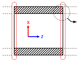
One use of MPCs is a master and slave situation: the displacement at node X (the slave node) is needed to be the same as at node Y (the master node). In Figure 1, a portion of a long vessel is modeled. The left side uses symmetry boundary conditions; this restrains the model in the Z translation and simulates the portion of the tank to the left. For a long vessel, the portion of the tank to the right side of the model forces those nodes to remain in a plane. A symmetry boundary condition would work except that these prevent axial growth or contraction in the tank. Instead, MPCs are used to indicate that the Z displacement of all the nodes are equal (but not necessarily 0). Similarly, temperatures in a thermal analysis and voltages in an electrostatic analysis can be the basis of MPCs.
|
|
Detail:
|
|
|
Z symmetry conditions restrain the left face. Those nodes do not move in the Z direction. |
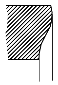
MPC conditions restrain the right face to remain in a plane; the nodes move together in the Z direction. |
Without MPC or other boundary conditions, the nodes on the right face are free to deflect due to the loads. This does not accurately simulate the portion of the vessel not included in the analysis. |
|
Figure 1: Use of Multi-point Constraint |
||
The input for multi-point constraint is an equation with the following format:
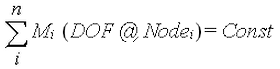
where
- i is the ith term of the equation
- M i is a multiplier for term i of the equation
- DOF@Node i is a degree of freedom (DOF) at a specific node for term i. The type of DOF depends upon the analysis type (translational or rotational displacements for linear structural analyses, temperature for thermal analyses, and voltage for electrostatic analyses).
- n is the number of terms in the equation
- Const is the constant that the equation equals. This value is often zero.
If the equation involves any units, they are written using the Model Units. The MPC equations do not use the Display Units.
Enter the MPC Equation
- In the FEA Editor, write down the vertex numbers and associated DOF(s) required for the MPC equations. To get the vertex numbers, use the Selection
 Select Vertices to select one vertex, then right-click and choose Inquire. (Or, just holding the mouse pointer over a vertex with show the properties in a tool tip.)
 - For all supporting analysis types, the Multi-Point Constraint command is found in the Setup tab of the ribbon.
- For linear structural analyses, the command is in the pull-out portion of the Constraints panel.
- For thermal analyses, the command is in the pull-out portion of the Thermal Loads panel.
- For electrostatic analyses, the command is in the pull-out portion of the Loads panel.
Multi-Point Constraint. Use the Define Multi-Point Constraints dialog box to enter all the terms of the previous equation. - Click the Add button to create a new constraint equation; the name of the equation is automatically filled in. Or use the Equation name drop-down menu to select an existing equation to edit.
- Specify the constant of the equation in the Constant field. (Const in the above equation.)
- Use the Add Row button to add as many rows to the spreadsheet as required to specify each term of the equation. In each row, enter the Multiplier and Vertex ID ( the vertex number written down from step 2) and the appropriate DOF (degree of freedom). Use the available drop-down list for linear analyses. The DOF is fixed for thermal and electrostatic analyses (DOF = Temperature and Voltage, respectively). Note: If a vertex is assigned to a local coordinate system, the DOF selected is also in the local coordinate system. For example, X translation refers to the radial translation direction in a cylindrical coordinate system, Y translation refers to the tangential direction, and so on.
- Choose the Solution method and set the Penalty multiplier (the Penalty multiplier is used for the Penalty method). You can select from the following Solution methods:
- Automatic
- Penalty Method
- Condensation Method
Note: You can find recommended values for the Penalty multiplier in the respective Set Up topics. Search on "Penalty multiplier" for quick access to the topics.Note: The solution method you select in the Define Multi-Point Constraints dialog box becomes the method used for all features that include MPCs. These features include, but are not limited to, cyclic symmetry, frictionless constraints, smart bonding, and user-defined MPCs. For example, if you want to use the Penalty Method to solve all your analyses involving smart bonding, you can override the default condensation method by selecting Penalty Method in the Define Multi-Point Constraints dialog box. - Click the OK button to close the dialog box.
- Run the analysis.
Compatibility Note: Versions 20 through 20.4 SP1
The input used to store the MPC data in versions 20 through 20.4 SP1 is no longer compatible. To recover the original input, edit the file DS.CST.BAK located in the design scenario folder (for example, modelname.ds_data\1). This gives the original MPC equations. The node numbers need to be converted to the corresponding vertex numbers, and then the equations need to be re-entered through Add Multi-Point Constraint. The format of the .CST.BAK file is as follows:
| #_equations, max_n |
Two numbers: the number of equations in the file (#_equations), and the maximum number of terms in any of the equations (max_n, not counting the constant that the equation equals). Both numbers must be integers. |
| #_terms(1) |
Number of terms in equation 1. This must be an integer. |
|
node(1), DOF(1), M(1) node(2), DOF(2), M(2) node(3), DOF(3), M(3) node(#_terms), DOF(#_terms), M(#_terms) |
Three numbers per line and #_terms lines of numbers. The three numbers are the node number (node(i)), the degree of freedom at the node (DOF(i)), and the multiplier for the term (M(i)). The multiplier must be a real number and the other two must be an integer. The valid numbers for DOF(i) are as follows: 1 = X translation 2 = Y translation 3 = Z translation 4 = X Rotation 5 = Y Rotation 6 = Z Rotation |
| Constant(1) |
The constant value for equation 1. This number must be a real number. (1.00 or 1.0E0 instead of 1) |
|
The above three sets of lines [#_terms; node(i), DOF(i), M(i); Constant] repeat for each MPC equation, number 2 through #_equations. |
Example
Analyze the gear train in Figure 2. Instead of trying to model the gears with beam elements to mimic the rotational connection, use Multi-Point Constraints. For the gears, Radius1*rotation1 = -Radius2*rotation2. So the MPC equation is Radius1*rotation1 + Radius2*rotation2 = 0. For the dimensions and vertex numbers given, the input for the MPC is as follows:
Equation 1
Constant = 0
|
Multiplier |
Vertex ID |
DOF |
|
3 |
12 |
X Rotation |
|
9 |
18 |
X Rotation |
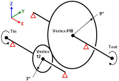
Figure 2: Gear Train Analyzed with Beam Elements