- A variable load is a load that is applied over an area; a surface. A variable load can be applied in any direction specified by a vector or can be applied normal to the surface.
- A function can be defined to control the magnitude of the load at different locations on the surface.
- The variable load is converted into equivalent forces and applied to the element nodes.
What Does a Variable Load Do?
Apply Variable Loads
If you have surfaces selected, you can right-click in the display area and select the Add pull-out menu. Select the Surface Variable Load command. You can also access this command via the ribbon (Setup  Loads Variable Pressure).
Variable loads can be applied to any meshed surface: specifically on plates, shells composites, membranes, bricks, tetrahedra, 3D kinematic, and 3D hydrodynamic elements. They are not available for 2D elements.
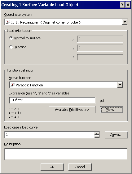
Select the coordinate system that the variable load follows in the Coordinate system drop-down menu. All local coordinate systems defined in the FEA Editor environment is listed in addition to the global coordinate system. For example, if you want a surface variable load to start at zero at an edge of a surface, you should create a coordinate system that has the origin at one of the nodes along that edge. Select that coordinate system in this drop-down menu.
If the direction of the variable load will always be normal to the surface, select the Normal to surface radio button in the Load orientation section. If the variable load is applied in a constant direction, select the Traction radio button in the Load orientation section and define the direction as a vector in the X, Y, and Z fields.
When creating a new load, the Active function drop-down menu is set to New function. Either type a name to create a new function, or use the drop-down menu to select an existing function. If you change the parameters of the function, the changes are applied to every variable load in the model that uses that function.
Define the function in the Expression field. The equation represents a pressure applied to the surface. Use the variables r, s, and t in the expression; note how the definition of these variables changes depending on the coordinate system as shown on the dialog box. You can use basic operators such as + - * / ( ) and ^. Click the Available Primitives >> button to access several common functions.
Click the View button to see a graphical view of the load along a specific direction. You can select the radio button for the variable plotted along the abscissa axis (the X axis) of the graph. Define the other two coordinates if they are used in the expression. For example, if you have a load that increases linearly in the X direction, select the X radio button. It generates a straight line at a constant slope. Since the load does not vary in the Y or Z directions, it does not matter what values are entered for these coordinates. If the expression were 5*(X+Y) and you chose the X radio button to see how the pressure changes versus the X coordinate, then you need to enter a specific value for Y. The graph will show how the pressure varies in the X direction based on the entered Y coordinate. You can view the graph at different Y coordinates by changing the coordinate and pressing the Recalculate button.
In the Load case / load curve field, specify the load case in which you want the variable pressure placed (for linear analyses). If you are going to perform a transient stress (direct integration) analysis or a nonlinear analysis, this field contains the number of the load curve that will be used to control the variable pressure throughout the analysis.
Since the variable load is converted into nodal forces, the load in the Results environment may not appear to follow the function exactly. If the mesh is not evenly spaced, numerous forces of low magnitude may be applied in an area with a fine mesh and fewer forces of higher magnitudes may be applied in an area with a coarse mesh. Also, nodes that are not shared by multiple elements have a force with a lower magnitude than the others. The node gets a force applied from each element that it is shared by.
- When modifying a surface variable load, it is suggested to use the same Display Units as when the load was created. (Right-click the Display Units in the Unit System branch of the tree view and choose Activate.) Viewing the load in other units shows conversion factors since the equation must give the same result regardless of the units.
- For example, the equation: 0.0361 [lbf/in^3] * (12.5 [inch] - Z [inch]) represents a hydrostatic pressure in units of psi, increasing in the negative Z direction, starting at an elevation of Z=12.5 inches. (The units are shown in brackets [ ] in this example to make the discussion easier to follow; the software does not show the units for each term.) When the Display Units are set to SI and the load is modified, the equation is now 0.0361 [lbf/in^3] * (12.5 [inch] - 39.37 [inch/m] * Z [m]) * 6894.8 [Pa/psi]
- A quick hand calculation shows that these two equations give identical pressures in the respective units, but interpreting the second equation can be more challenging.
Example of Variable Load
We will set up and view a model of a 5 inch cube with the following variable loading.
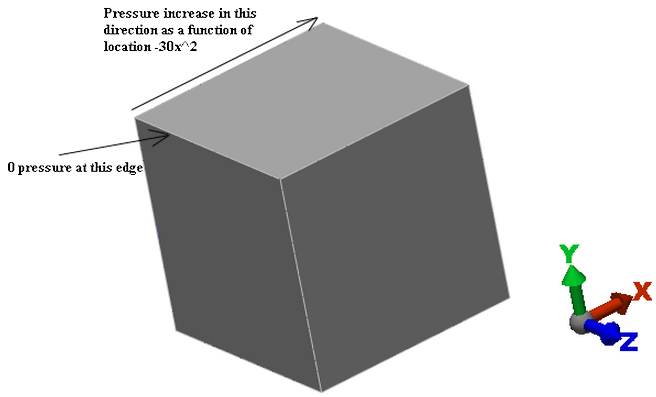
First we should set up a rectangular local coordinate that has the origin along the edge of 0 pressure and the local X axis parallel to the direction of increasing load. Next we select the surface and right-click in the display area and select the Add Surface Variable Load command. The variable load parameters should be set as shown below.
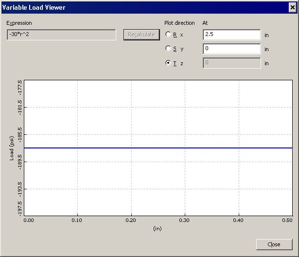
Click the View button to show the following graph along the X direction.
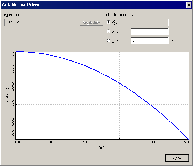
Since the model does not vary in the Y or Z directions, the values in the y and z coordinate fields are not relevant. For verification purposes, the value half way along the surface should be constant at -30*(2.5)^2=-187.5. Select the T radio button and type 2.5 in the R field. Press the Recalculate button. The following graph should appear.
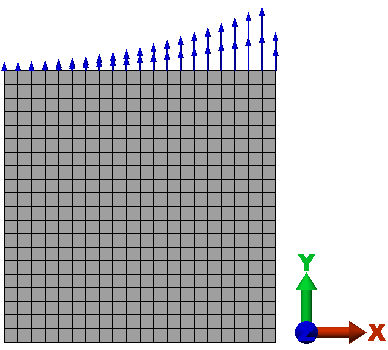
If we view the model in the Results environment, it appears as shown in the following image. The reason for the shorter arrows along the edge is because there are fewer elements sharing those nodes.