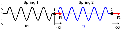
In one form or another, Finite Element Analysis (FEA) comes down to solving a set of equations. Take the simple two spring model shown below, where F1 and F2 are the applied loads, K1 and K2 are the stiffness of the springs, and X1 and X2 are the deflections of each end. Keep in mind that either of the applied loads can be zero, but each one is a known value. The force developed in each spring due to elongation is unknown, but it can be calculated from the direct formula F = k*x. Considering that spring 1 elongates by the amount X1 and spring 2 elongates by the amount (X2-X1), we can write the equation for the sum of the forces at each node:
| F1 - K1*X1 + K2*(X2-X1) = 0 | node 1 |
| F2 - K2*(X2-X1) = 0 | node 2 |
Rearranging the equations gives:
| F1 = (K1 + K2)*X1 - K2*X2 | node 1 |
| F2 = -K2*X1 + K2*X2 | node 2 |
These equations can be expressed in matrix form as follows:

or in shorthand notation, {F} = [K]{X}.
How the matrix of equations is solved in FEA is the task of the solver. As computer hardware and computational techniques evolve, new solvers are added to the software. Each analysis type has various solvers to choose from. In many cases, the default option is Automatic, in which case the software chooses the solver best suited for the analysis (usually based on the size of the model (the number of equations). The following discussion gives the general methodology of each type of solver.
Depending on how the elements are connected together, the stiffness matrix [K] is generally very sparse. Many of the entries are zero. Since a value of zero does not contribute to the solution, most solution techniques are programmed in some fashion or another to ignore the zero terms. One method may use a small amount of memory to store the matrix but require optimization to achieve the least amount of memory, where as another method uses more variables to store the matrix (and hence require more memory) but be faster overall.
Next, the solution to the set of equations will determine how long the analysis requires. There are direct solution methods that are guaranteed to give a solution, provided the model is set up properly (static stress model is properly constrained, steady state heat transfer model has a source of heat and way to remove the heat, and so on). Techniques such as Gauss Elimination and matrix inversion are simple examples of direct solution methods. Then there are indirect solution methods in which the solution is assumed. By substituting the assumed solution into the system of equations, a better estimate is obtained for each unknown. This process is repeated until the solution no longer changes; hence, these techniques are known as iterative solution.
Finally, the stiffness matrix is generally symmetric in FEA. In these cases, only the terms on and above the diagonal need to be stored. This reduces the memory requirements and number of operations to solve the matrix. When an effect is included which causes the matrix to be unsymmetric (such as body-to-body radiation in a heat transfer analysis, or an actuator element in a Mechanical Event Simulation), the entire matrix needs to be stored and operated upon. The solution will be longer in such cases.
Below are the general solvers available. Each one may have variations for a particular analysis type. For example, modal analysis has an iterative solver (subspace) which is a variation of the iterative solver available in linear static stress (AMG, or Algebraic MultiGrid). The type of solver used in the analysis is set from the Setup Model Setup Parameters(or right-click the Analysis Type entry in the tree view and choose Edit Analysis Parameters).
Sparse Solver
- Provides a direct solution to the matrix.
- The bandwidth is not optimized, so time spent performing this operation is saved.
- Instead of storing the entire matrix, only the nonzero terms are stored. (This is where the terminology of Sparse solver comes from.)
- Although fewer terms from the stiffness matrix are stored, more variables are required to store the position of the nonzero terms. Thus, the sparse solver requires more memory than the other solvers.
- The sparse solver is the fastest solution for midsize models.
Iterative Solver
- Provides an indirect solution to the matrix. Thus, the user must specify the maximum number of iterations to be performed, and a convergence criteria to decide when the solution has converged. There is no guarantee that the solution to the matrix will be found within the number of iterations specified.
- Since the iterative solver needs to starts with an initial guess, some of the processors have a preconditioner. This provides more options to choose from to get the model to solve efficiently.
- The bandwidth is not optimized, so time spent performing this operation is saved.
- The iterative solver requires less memory than the sparse solver.
- When able to converge, the iterative solver is the fastest solution for large models. Large depends on the analysis type. For linear static stress, 150,000 equations (or degrees of freedom) is large. For fluid flow, 50,000 equations may be large. Attention: The accuracy of the solution depends on the convergence tolerance; a smaller tolerance will result in a more accurate solution but may take more iterations. As with any iterative solution, the results should be checked to confirm that they meet the appropriate accuracy. In some cases, performing the analysis twice with a different convergence tolerance is the best way to confirm the accuracy.Note: The iterative process to solve the matrix is one level of convergence required. This provides the solution to the set of equations. If the analysis is also nonlinear, then the problem needs to be solved repeatedly to converge to the physical solution. For example, radiation causes the equations being solved to be nonlinear. This requires multiple iterations to find the solution to the nonlinear equations. (Normally, the equations are linear and require only one solution.) Do not confuse the iterative process to solve the model with the iterative process to solve the system of equations.Tip: If the analysis fails to converge with the iterative solver and gives the message Matrix might be not positive definite or Condition of the preconditioned system =, the problem may be due to a statically unstable model. In a static stress analysis, make sure that all components are statically stable. If the model includes contact, see the suggestions on the page Setting Up and Performing the Analysis: Performing the Analysis: Performing A Linear Analysis: Performing Analyses with Gap Elements.