Ball in a Box with Body-to-Body Radiation

Problem Statement: A 0.5-m diameter hollow ball is inside a 0.8-m cubic box operating in a near vacuum as shown in the following figure. One side of the box is maintained at 150°C. The ambient temperature is -80°C. The conductivity for both objects is 3 W/(m°C). The thickness of the walls of the ball and the box is 0.001m. The ball has an emissivity of 0.5. The box has an emissivity of 0.8.

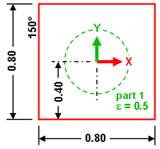
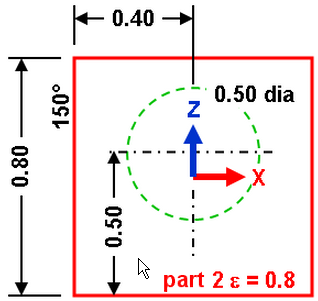
Ball in a Box in the XY view and XZ view

Find: Temperature of the ball.

This example only covers setting up and performing the analysis. For instructions on building the model, see Ball in a Box with Body to Body Radiation Model. If you have not built the model, you can open the b2brad_input.ach file in the Models subfolder of the Autodesk Simulation installation directory.

Since the properties of the ball (Part 1) and box (Part 2) are identical, they are defined simultaneously.

1. Click the heading for Part 1 in the tree view. Hold down the Ctrl key and click the heading for Part 2. Everything in the display area is selected.
2. Right-click one of the items (or anywhere in the display area) and select Edit Element Type Plate.
3. Right-click one of the items (or anywhere in the display area) and select Edit Element Data. Type 0.001 in the Thickness field. In the Element Normal section, type 0.1 in the Z-coordinate field. This point is used to define which side of the plate elements is the top and which is the bottom. The top side of the plates is the side opposite from this point. The outside of the sphere and box are defined as the top side of the plate elements. (Note: Any coordinate inside the sphere is acceptable). Click OK.
4. Right-click one of the items and select Edit Material. With [Customer Defined] highlighted, click Edit Properties. Type 3 in the Thermal conductivity field and click OK twice. (Thermal conductivity is the only material property required for a steady-state analysis.)
5. Save the model.
6. With nothing selected on the model, right-click the display area and select the Body-to-Body Radiation command.
7. First, define which surfaces can participate in the body to body radiation and the properties of those surfaces. (See the tips at the end of this topic.) Click Define surfaces. Click Add Surface to specify which surfaces you want to be in radiation Surface 1 (the ball). Select the 1 option in the Part number drop-down menu to select the ball, the All option in the Surface number drop-down box, and the Both option in the Plate element side drop-down menu. The ball radiates to itself across the inside of the ball (the bottom side of the plate) in addition to radiating out to the box. Click OK.
8. The data that you specified for radiation Surface 1 (the ball) appears in the Definition of Surface section. Type 0.5 in the Temperature independent emissivity field.
9. Click Add Surface again to define radiation Surface 2 (the box). Select the 2 option in the Part number drop-down menu to pick the box, the All option in the Surface number, and the Bottom option in the Plate element side drop-down menu.  Radiation from the outside of the box to the ambient is handled with a surface load. Click OK.
10. The data  specified for Surface 2 appears in the Definition of Surface section. Type 0.8 in the Temperature independent emissivity field. Click OK.
11. Now that the surfaces involved in radiation are defined, assign them to a radiation enclosure. On the Enclosures tab, click Add Surface in the Surfaces section. Click OK to add Surface 1 to Enclosure 1. Click Add Surface again. The second surface appears in the drop-down menu. Click OK to add Surface 2 to this enclosure. Each defined surface can participate in only one enclosure.
12. Select the Included option in the Shadowing drop-down menu. In the Ambient temperature drop-down menu, select the Time-independent option and type -80 in the Ambient temperature value field. Mathematically, the view factors may not sum to a value of 1. Always enter a reasonable ambient temperature.
13. Because the radiating surfaces are close to each other (especially along the edges of the box), use the more accurate view factor calculation method. Click the Parameters tab, then set the View factor calculation method to String rule/contour integration.
14. Click OK to exit the Body-to-Body Radiation dialog box.
15. Now we must define the convection surface load to keep the left wall at 150°C. Click the + next to the Surfaces heading under Part 2. Right-click the Surface 2 heading and select Add Surface Convection Load. Type 1000 in the Temperature Independent Convection Coefficient field and type 150 in the Temperature field. This coefficient should be large enough to keep the temperature at 150°C. (The wall temperature is calculated, and it is not exactly 150°C. It is close depending on the magnitude of the convection coefficient. After obtaining the results, remember to check that the wall temperature is close enough to 150°C to satisfy any requirements.) Activate the Apply load to both sides check box to help maintain the temperature. Click OK.
16. The outside of the box radiates to ambient temperature. Right-click the Surface 1 heading in Part 2 and select Add Surface Radiation Load. Type 0.8 in the Function field and type -80 in the Temperature field. The radiation function is the view factor, 1, times the emissivity, 0.8, for all the elements on the selected surfaces. Click OK. Surface 2 does not need radiation in this situation since it is being held at 150°C.
    Note: You could use body-to-body radiation outside of the box. However, since you know that the outside surfaces do not see anything other than ambient, body-to-body radiation wastes computational time. In a large model, the view factor computation can be significant.
17. Now we must set up the analysis parameters. Right-click the Analysis Type heading of the tree view and select the Edit Analysis Parameters command.
18. Click the Advanced tab. Activate the Perform check box so that the nonlinear iterations are performed during the analysis. In the Criteria drop-down menu, select the Stop when corrective norm < E1 (case 1) option to ensure that the temperature change between successive iterations is less than the Corrective tolerance. Type 90 in the Maximum number of iterations field, type 0.5 in the Corrective tolerance field and type 0.3 in the Relaxation parameter field.
    Note: You can also try other values for the convergence parameters. A large relaxation parameter can lead to an unstable solution. Also, while a corrective tolerance of 0.5 degrees can seem large, the results show that the actual convergence is much smaller.
19. To aid the convergence, enter an estimated temperature of the nodes for the first iteration. As a quick approximation, set all the nodes to 60°C. Click the Options tab and enter 60 for the Default nodal temperature.
20. Click OK to assign the Analysis Parameters.
21. Select Analysis Analysis Run Simulation to perform the analysis.
22. The temperature profile appears by default in the Results environment when the analysis completes. The results of the intermediate iterations are visible in the Results environment while the analysis runs. Thus, you can see how the results are converging or diverging as the solution iterates.

    Visually, the hot face of the box is close to 150°C. The convection coefficient was large enough to hold the wall near the preferred temperature. (If greater precision is required, then use a larger convection coefficient.)

23. You can see the effects of the shadowing on the wall opposite the 150°C. Note the cool spot in the upper center area.
24. When an iterative method is used to solve a problem, check the log file and review the final convergence. Click the Report tab and click Log in the tree view under the Steady-State Heat Transfer branch. The log file displays in the window. Scroll down to the non-linear iterations section, where the history is like the following table.  

    * * * *BEGIN NON-LINEAR ITERATIONS
    Nonlin Iter.	Incr. Norm(T)	Incr. Norm(Q)	Rel. Norm(T)	Rel. Norm(Q)
    1	1.134E+02	1.024E+02	2.630E+00	3.333E+00
    6	8.471E+00	1.039E+02	1.351E-01	4.422E-01
    11	2.025E+00	2.997E+01	3.033E-02	9.484E-02
    16	3.682E-01	7.019E+00	5.461E-03	2.085E-02
    21	6.236E-02	1.504E+00	9.233E-04	4.409E-03
    25	1.488E-02	4.227E-01	2.203E-04	1.236E-03
    **** END NON-LINEAR ITERATIONS
    **** CONVERGED SOLUTION OBTAINED

Iteration (Iter) 25 indicates that the change in temperature (Incr. Norm (T)) was 0.0149°C. It is considerably smaller than the corrective tolerance specified (0.5°C). The solution is well converged. (When body to body radiation is involved, the corrective tolerance is applied to the incremental norm in temperature (T) and to the incremental norm in heat flux (Q). In this case, the heat flux required more iterations to converge than the temperature.)

Tip:

Here are some tips when working with body to body radiation problems:

• A radiation surface is one surface (or many surfaces) of a part that is involved in radiation. It is created first using Define Surfaces.
• After defining which radiation surfaces are involved, assign them to an enclosure. Each enclosure is a set of radiation surfaces that radiate to each other (and optionally to the ambient) but to no other surfaces.
• Consider whether shadowing is needed since it adds considerably to the computational effort. Shadowing is needed if the radiation from one element in the enclosure would pass through another element in the enclosure to get to a third element. For example, radiation from the left side of the box passes through the ball and sees the right side of the box if shadowing is not included.
• Set the default nodal temperature to help reduce the number of iterations. Without a default temperature, the model starts at 0 degrees and may require more iterations to reach the final condition. The temperatures of the nodes can be set individually by adding a Nodal Temperature to selected vertices. Any node without a nodal temperature uses the Default nodal temperature set under the Analysis Parameters: Options tab.
• Set up the nonlinear iteration parameters on the Advanced tab of the Analysis Parameters. In general, larger nonlinear effects, like radiation, require smaller relaxation parameters to avoid divergence.
• Review the log file for the non-linear convergence history. For example, a large incremental temperature norm may indicate an inaccurate solution. To analyze the model again, the relaxation parameter can be tweaked to speed convergence (or reduce divergence), or a different tolerance may give a faster runtime or a more accurate result.

An archive of this model (b2brad.ach) without results is located in the Models subfolder in the Autodesk Simulation installation directory. Analyze the model to view the results.