Activating the command: Results Options Other Tools Combine Load Cases in the Results environment.
Use the Combining Load Cases dialog to add the results from multiple models (or from multiple load cases in a single model) to create a new set of results. In addition to the obvious situation of creating new load scenarios from existing results, it is often easier and faster to run separate analyses and combine the results to get the new combinations instead of putting all the combinations in one run. The results that are combined are the displacements, reaction forces, and stresses, provided that these results exist for all the models/load cases being combined. For example, both linear static stress and modal analyses have displacement results, so the combined results will include the displacements (even though these displacements represent different things in each model). But since modal analysis does not have stress or reaction forces, the combined results will not have stresses or reaction forces.
In the process of combining the results, you can specify the following:
- model to use
- load case from the analyzed model to use
- scale factor (multiplier) to be applied to each analyzed load case
- take the absolute value of the analyzed load cases
- create an SRSS (square root sum of squares) of the analyzed load cases
For example, imagine the following ten sets (load cases) for a design:
- gravity in X-direction + nodal forces
- gravity in X-direction + pressure
- gravity in X-direction - pressure
- gravity in X-direction + nodal forces + pressure
- gravity in X-direction + nodal forces - pressure
- gravity in Y-direction + nodal forces
- gravity in Y-direction + pressure
- gravity in Y-direction - pressure
- gravity in Y-direction + nodal forces + pressure
- gravity in Y-direction + nodal forces - pressure
Perhaps the pressure represents the wind, and therefore it needs to be analyzed in a positive and negative direction, and the nodal forces are live loads. Since the gravity, nodal forces, and pressure repeat in the above load cases, the following models and load cases can be analyzed:
| Model | Load Case | Applied Load |
|---|---|---|
| Design_X | 1 | gravity in X-direction |
| 2 | nodal forces | |
| 3 | pressure | |
| Design_Y | 1 | gravity in Y-direction |
and combined as follows:
| Applied Load | New Load Case | Models to Combine (scale factor * model load case) |
|---|---|---|
| gravity in X-direction + nodal forces | 1 | (1)*(Design_X LC 1) + (1)*(Design_X LC 2) |
| gravity in X-direction + pressure | 2 | (1)*(Design_X LC 1) + (1)*(Design_X LC 3) |
| gravity in X-direction - pressure | 3 | (1)*(Design_X LC 1) + (-1)*(Design_X LC 3) |
| gravity in X-direction + nodal forces + pressure | 4 | (1)*(Design_X LC 1) + (1)*(Design_X LC 2) + (1)*(Design_X LC 3) |
| gravity in X-direction + nodal forces - pressure | 5 | (1)*(Design_X LC 1) + (1)*(Design_X LC 2) + (-1)*(Design_X LC 3) |
| gravity in Y-direction + nodal forces | 6 | (1)*(Design_Y LC 1) + (1)*(Design_X LC 2) |
| gravity in Y-direction + pressure | 7 | (1)*(Design_Y LC 1) + (1)*(Design_X LC 3) |
| gravity in Y-direction - pressure | 8 | (1)*(Design_Y LC 1) + (-1)*(Design_X LC 3) |
| gravity in Y-direction + nodal forces + pressure | 9 | (1)*(Design_Y LC 1) + (1)*(Design_X LC 2) + (1)*(Design_X LC 3) |
| gravity in Y-direction + nodal forces - pressure | 10 | (1)*(Design_Y LC 1) + (1)*(Design_X LC 2) + (-1)*(Design_X LC 3) |
Setting up two models or design scenarios with a total of 4 load cases and using the Load Combination is less work for you than setting up two models with a total of ten load cases. Also, once the base results are created in the two models, they can be combined and scaled quickly at a later time without rerunning the analysis of the models.
The input in the last column of the above table is the information entered into the Combining Load Cases dialog.
- The models being combined must be identical in geometry. The node numbering, the part numbering, and the element numbering must match in all models. Furthermore, the boundary conditions and material properties should match in all models to represent a valid combination, but there may be situations where this is not necessary.
- The load combination uses the principle of superposition which states that a result (stress, displacement, and so on) due to different loads may be computed separately and added algebraically. This is not proper for some analysis types or some load cases (such as the resultant from a vibration analysis) in which the results being added have a magnitude but no direction. The SRSS (square root sum of squares) process used for the resultant has lost whether the result is positive or negative. Caution is suggested when combining such results.
General Steps
The basic steps to combine the results from multiple models are as follows:
- Analyze all the models.
- While viewing the results of one of the models, use Results Options Other Tools Combine Load Cases.
- Specify the name of the model to be created, the file with the combined results. (See Specifying the New Results File: below.) The name entered is also used to create a folder with the same name, and the model is placed in the new folder.
- Specify the existing results to combine and the multiplier for each. (See Specifying the Models to Combine: below.)
- Add a new load case if the combined model is to have multiple load cases. (See Specifying the New Load Case: below.)
- Repeat step 4 for each load case.
- Run the load combination utility by clicking the Combine load cases button. (See Creating the Combined Results: below.)
- Use
 Open to open the newly created results. (See Viewing the Combined Results: below.)
Specify the New Results File
The path and filename of the new model with the combined results are shown in the text box Path and name of file containing combined load cases. Click the button to use a standard Save As dialog. The combined result files are placed into a folder with the same entered name. For example, clicking the button and entering a new name of my_combined_results will place the results in a file named my_combined_results.fem located in a folder named my_combined_results. The folder is created if it does not exist.
Specify the New Load Case
Since the new results can contain multiple load cases, the left half of the Specification of New Load Cases section is used to create and display the new load cases. The Load case in combined model pull-down is used to set which new load case is being shown in the Composition of New Load Case spreadsheet. New load cases are added to the new results by clicking the Add new load case button. In the previous example, you click the Add new load case button 9 times to get the 10 load cases required. The Composition of New Load Case spreadsheet needs to be filled out before adding a new load case.
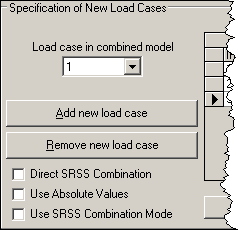
Figure 1: Load Cases to Create(continued in Figure 2)
Use the Remove new load case button to remove the new load case that is currently displayed.
Options for Combinations
There are numerous options for combining the results. These are the check boxes on the left half of the dialog. The options and effects are as follows:
- The Direct SRSS Combination option will perform a square root sum of squares (SRSS) operation on the analyzed load cases specified in the Composition of New Load Case spreadsheet. Each result component in the combined results calculates as follows:
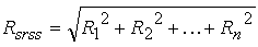
where
- R is any results in the binary results file (displacements, rotations, primary stresses).
- R1 is the result component for the analyzed load case specified on row 1 of the spreadsheet, R2 is the result component for the analyzed load case specified on row 2 of the spreadsheet, through row n.
- Rsrss is the square root sum of squares result and written to the new model.
The Multiplier for each analyzed load case must be 1 to perform the combination when using this option.
Secondary results (principal stresses, and other stresses calculated from primary stresses) are calculated for each analyzed load case shown in the spreadsheet and then combined using the above formula.
The option Direct SRSS Combination is not available if more than one output load case is specified for the combined model.
Tip:- The Direct SRSS Combination method can be used to satisfy the missing mass method described in the U.S. Nuclear Regulatory Commission's Regulatory Guide 1.92, Combining Modal Responses and Spatial Components in Seismic Response Analysis (rev 2, July 2006). For this requirement,
- Choose the resultant load case from a response spectrum or DDAM analysis.
- Choose one static stress result.
- In this situation, the combination is equivalent to R I = [R rI 2 + R pI 2 ] 0.5 from the NRC Regulatory Guide.
- The Use Absolute Values option will take the absolute value of the analyzed load cases shown in the spreadsheet, multiply by the Multiplier, and add the terms together. It is intended to give a more conservative result in cases where the terms with different signs are added. Attention:
- The Load Combination Utility takes the results in the binary result file, scales them based on the multiplier, and adds the results together. So, some combined secondary results (results based on other values) may not match the hand-calculated results based on the combined primary results. The combined results may be further manipulated in the Results environment to display the chosen result (von Mises stress for example).
- The sum of the absolute values, when the Use Absolute Values check box is activated, and further processing by the Results environment may lead to unexpected results. Interpret the results carefully to make certain they are providing a meaningful result when the Use Absolute Values is activated.
- For example, the axial stress in beam elements (Results: Stress: Beam and Truss: Axial Stress) is a calculated result; it is not a result read directly from the binary file. Thus, if other results used to calculate the axial force are now always positive, the calculation of the axial stress can be incorrect.
- The Use SRSS Combination Mode option will perform a square root sum of squares (SRSS) operation on the analyzed load cases specified in the Composition of New Load Case spreadsheet. Each result component in the combined results calculates as follows:
where
- R is any displacement result (displacements, rotations) in the binary results file
- R1 is the result component for the analyzed load case specified on row 1 of the spreadsheet, R2 is the result component for the analyzed load case specified on row 2 of the spreadsheet, through row n. Each R is multiplied by the Multiplier value before squaring.
- Rsrss is the square root sum of squares result and written to the new model.
After the displacements are combined, the Stress Calculation Utility (mknso.exe) is executed. All stress results are calculated based on the element stiffness and combined displacements.
Attention: The method of calculating the stresses from the combined SRSS of the displacements may lead to inaccurate results for some models.The option Use SRSS Combination Mode is not available if more than one output load case is specified for the combined model.
- When none of the above options are selected, all results in the binary files (displacements, rotations, stresses) are multiplied by the Multiplier and added together (linearly combined). This is the definition of superposition
Specify Models to Combine
The right half of the Specification of New Load Cases section is used to indicate which previously analyzed models to combine, which load case to use from the models, and the multiplier used for each load case. Use the Add Row and Delete Row buttons to add or delete rows to the spreadsheet to specify additional model results to combine.
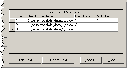
Figure 2: Models to Combine(continued from Figure 1)
Clicking in the Results File Name or Load Case cell of the spreadsheet will give a new dialog window. Use the Select Results File button on the new dialog to indicate which results file to use in the combination. Be sure to set the Files of type: drop-down arrow as necessary for the type of results to select. (Also, keep in mind that the results are located in the design scenario folder under the model's ds_data folder.) After the file is chosen, use the Existing load cases in file pull-down on the new dialog window to indicate which load case to use from the analyzed model. Click the OK button to fill the information into the spreadsheet.
Click in the Multiplier column of the spreadsheet to enter the multiplier for the chosen load case. The multiplier can be any value: positive or negative, whole number or fraction.
Create Combined Results
To perform the computations and create the combinations specified in the spreadsheet, click the Combine load cases button. A progress dialog window will appear; click the Combine button to begin the actual processing. After it completes, click the Log tab to view the feedback from the processor. Click the OK button to close the progress window, and then click the Done button on the Combining Load Cases dialog to close it.
View Combined Results
After creating the new load combination, use Open to open the new model and view the results. Be sure to set the Files of type on the Open dialog to Autodesk Simulation Results (*.fem). (The Load Combination Utility only creates the result files; it does not create an FEA model file.) See the tip below for the location of the model to select with the Open dialog.
If the default Autodesk Simulation FEA Model (*.fem) file is opened, then an empty model will appear in the FEA Editor environment: no geometry, no part information. Switch to the Results environment in this case to see the combined results.
The file and folder structure for the combined results model is as follows:
| |
The folder specified by the user for the new results file. This is where the combined model is saved. | |||
| combined.clc | The Combined Load Case file (.CLC) containing the input. In this example, the user specified the name as combined. | |||
| |
A folder created by the load combination software which contains the combined model results. | |||
| combined.fem | The Autodesk Simulation Results (*.fem) file. This is the file to open. | |||
| |
A folder created by the software to hold each design scenario data. | |||
| |
Folder for design scenario number 1. The user normally does not need to access any data below this folder for a combined model. | |||
|
ds.asd ds.do3 ds.lg3 ds.ns3 |
Files with the results for design scenario 1. | |||
|
|
ds.mod | The .MOD folder for design scenario 1. | ||
When either the Direct SRSS Combination option or the Use SRSS Combination Mode is used, the combined results file will have the following features:
- The analysis type will be Response Spectrum.
- The results will include the results from all the analyzed load cases and the SRSS result. Use Results Options Analysis Specific Resultant in the Results environment to toggle between which results are shown.