Any nodal load or constraint that is applied along a specific direction is applied in a coordinate system. By default, all loads and constraints are applied in the global coordinate system. Sometimes this is not adequate. For example, to restrict the translation of nodes along a specific vector that is not parallel to the global axes, you will not be able to accomplish this with boundary conditions. In this case, you can create a local coordinate system and apply it to nodes in the model. This local coordinate system will have local X, Y and Z directions. All loads and constraints applied to these nodes is applied along the local directions.
Results which have X, Y, and Z components can also be displayed in the Results environment using a local coordinate system.
- Loads are applied in the correct direction when based on an LCS.
- In the Results environment, results viewed in non-global directions, based on a defined LCS, are correct.
- However, constraints follow the global coordinate system for 2D elements, even when an LCS is defined and applied to the entities being constrained.
The following table summarizes which analysis types support local coordinate systems:
| Analysis Type | FEA Editor Environment | Results Environment |
|---|---|---|
| Linear | ||
| Static Stress with Linear Material Models | Yes | Yes |
| Natural Frequency (Modal) | Yes | Yes |
| Natural Frequency (Modal) with Load Stiffening | No | Yes |
| Response Spectrum | Yes | Yes |
| Random Vibration | Yes | Yes |
| Frequency Response | Yes | Yes |
| Transient Stress (Direct Integration) | Yes | Yes |
| Transient Stress (Modal Superposition) | Yes | Yes |
| Critical Buckling Load | No | Yes |
| Dynamic Design Analysis Method (DDAM) | No | Yes |
| Nonlinear | ||
| MES with Nonlinear Material Models | Yes | Yes |
| Static Stress with Nonlinear Material Models | Yes | Yes |
| MES Riks Analysis | Yes | Yes |
| Natural Frequency (Modal) with Nonlinear Material Models | No | Yes |
| Thermal | ||
| Steady-State Heat Transfer | not applicable | Yes |
| Transient Heat Transfer | not applicable | Yes |
| Electrostatic | ||
| Electrostatic Current and Voltage | not applicable | Yes |
| Electrostatic Field Strength and Voltage | not applicable | Yes |
Create the Coordinate System
Right-click the Coordinate Systems heading in the FEA Editor or Results environment tree view and select New to open the Creating Coordinate System Definition dialog box.
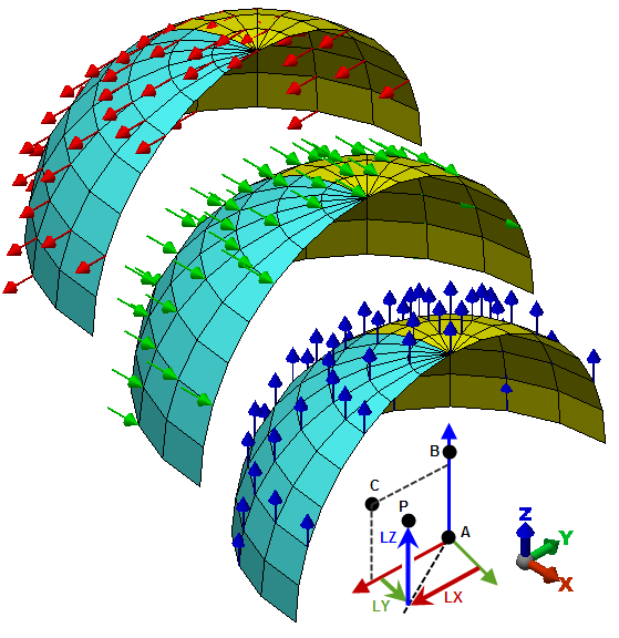
- Select the type of local coordinate system Coordinate System Type drop-down menu. The three available options are Rectangular, Cylindrical and Spherical. The image changes to depict how the three coordinates define the coordinate system. In all cases, the points A and B define the local Z axis. Points A, B, and C define a plane containing the local X axis. The local Y is determined by the right-hand rule. (See Table 2 also.)
- Define the three points, A, B and C. There are three methods.
- Type the global X, Y and Z coordinates of each point in the corresponding fields.
- Click Select A, Select B, or Select C for the appropriate point and then click a node in the display area. The coordinates of the selected node will appear in the corresponding fields.
- Click Interactive and then click three nodes in the display area. Axes appears as you select the nodes to depict the local axes that you are defining.
Assign Nodes to Coordinate System
Once a local coordinate system is defined, you can apply it to nodes in the FEA Editor by selecting the vertices (or a surface, part, and so on) and right-clicking in the display area. Select the appropriate coordinate system from the Coordinate Systems pull-out menu. The local axis appears on the nodes (in both the FEA Editor and the Results environment).
Different nodes can be assigned to different coordinate systems, but the same node cannot be assigned to more than one coordinate system.
Assign Loads and Constraints to Local Coordinate Systems
When a load such as a nodal force or boundary condition is added to a node assigned to a local coordinate system, the dialog box indicates to which coordinate system the node is assigned. The X, Y, and Z directions shown on the dialog box refer to the local directions of the coordinate system.
|
Coordinate System |
Figure |
Input Direction |
||
|
X |
Y |
Z |
||
|
Global (Default) |
- |
global X |
global Y |
global Z |
|
Rectangular |
2(a) |
Local X |
Local Y |
Local Z |
|
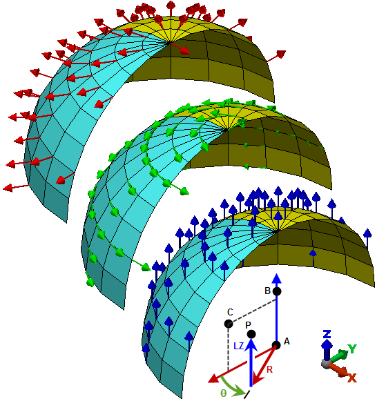
Cylindrical |
2(b) |
Radial |
Tangential (ϑ) |
Axial (local Z) |
|
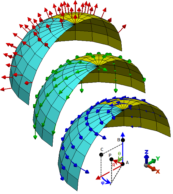
Spherical |
2(c) |
Radial |
Polar (ϑ) |
Tangential (φ) |
|
(a) Rectangular Coordinate System |
|
(b) Cylindrical Coordinate System |
|
(c) Spherical Coordinate System |
|
Figure 2: Local Directions for Coordinate Systems In each figure, the direction of local X, local Y, and local Z are shown on the three hemispheres from top left to bottom right. The local axes are shown in the bottom right hemisphere only. (All hemispheres are defined with the local coordinates at the centers.) The three points A, B, C that define the local coordinate system are entered using global X, Y, Z coordinates. Then an arbitrary point P is shown with its local coordinates. Although the coordinates of points cannot be entered using local coordinates, extending the coordinates to the point will show the direction of the loads and constraints, as shown by the nodal forces in each of the three hemispheres. |
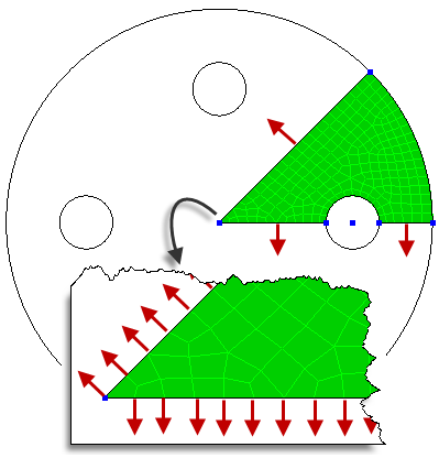
- Be aware that the radial and tangential directions for nodes on the axis (AB) of a cylindrical coordinate system are not uniquely defined. Likewise, the radial, polar, and tangential directions for nodes on the axis (AB) of a spherical coordinate system are not uniquely defined. The direction that the software chooses to represent these directions is arbitrary. Therefore, loads and boundary conditions in these directions should be avoided at nodes on the axis.
- Also, imagine a wedge-shaped model that represents a 1/8 section of a full disk (background portion of figure below). The edges are assigned to a cylindrical coordinate system, and symmetry boundary conditions are added to the edges so that the nodes cannot move in the tangential direction (red arrows in figure). The node at the center point is not restrained in two tangential directions as are required by the symmetry condition; it is only restrained in one direction (see inset in figure, which shows the tangential direction at all the nodes). You must place a radial and tangential constraint on this node.
- In the FEA Editor, separate and independent vertices are created at the junction between two parts. So, it is theoretically possible to create a different coordinate system on each vertex even though they are at the same coordinate. Likewise, a different nodal load can be applied to the two vertices, each on a different coordinate system.
- If the parts are bonded, then only one node is created between the parts when the Run Simulation or Check Model is used. One node cannot have two different coordinate systems. Therefore, vertices that are merged together to form one node will use the coordinate system and load from the vertex with the highest coordinate system ID. The other coordinate system and load are dropped from the analysis. The global coordinate system is considered to be ID 0, so it is the lowest.
View Results in a Coordinate System
Results which have X, Y, and Z components - such as displacements, reaction forces, and stress tensors - can also be displayed in the Results environment using a local coordinate system. If the coordinate system does not already exist, it can be created as described above. Then to view the results in the local coordinate system,
- Right-click the coordinate system in the tree view and choose Apply.
- View a result that has X, Y, and Z components, such as the displacements. The legend will indicate how the chosen result is interpreted in the new coordinate system (radial in a cylindrical system corresponds to Results: Displacement: X and so on).
- The results of the entire model are shown in the applied coordinate system regardless of which coordinate system the nodes are assigned to.

 OptionsResults tab. Click Individual FEA Objects Settings and scroll through the list to select Local Coordinate Systems. The Current: Show check box can be toggled to hide or show the icons.