Given: A flexible system with a moving base is composed of a body having a mass of 225 kg, a stiffness of the supporting structure of 35000 N/m, and a damping factor of 0.188. The base oscillates sinusoidally with an amplitude of 0.280 cm at the natural frequency of the system.
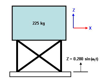 |
The physical assembly. The base is vibrated at the natural frequency of the structure. |
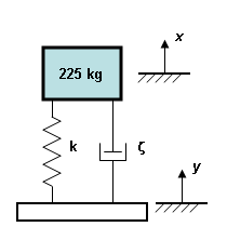 |
The equivalent representation. k = 35000 N/m ζ = 0.188 x and y are typical nomenclature in vibration text books for measuring the absolute motion of the mass and base. The lowercase italic nomenclature x and y indicate the position as a function of time. |
Find:
- The amplitude of the mass's displacement relative to the base.
- The absolute amplitude of the mass's displacement (displacement relative to a non-moving source).
Instead of modeling the entire support structure in detail, it can be represented with truss elements. (Recall that the stiffness of a truss element k is A*E/L.) The mass can be represented with a lumped mass added to the end of the truss. The moving base will be represented by a fixed boundary condition, and a ground motion or base acceleration load will simulate the oscillation of the base. The end of the truss element with the mass will have a boundary condition to restrict the mass to oscillating in the axial direction only.
Steps
- Perform a Natural Frequency (Modal) analysis to get the natural frequency. In addition to providing the frequency (as needed by the problem statement), the results of the modal analysis are use by the next two analysis types.
- Perform a Frequency Response analysis with base acceleration to get the quasi-steady state amplitude of the mass. Frequency Response simulates a sinusoidal load applied to the model.
- To check what happens to the system as it starts from 0 speed, perform a Transient Stress (Modal Superposition) analysis with base acceleration. Transient Stress uses a user-defined load curve to calculate the response of the model to a general load. Does a higher deflection occur during the transient?
Building the Model:
- Start a new FEA model.
- Set the analysis type to Linear: Natural Frequency (Modal).
- Since the oscillation is given in centimeters, lets select units of Newtons, centimeters, and seconds for the model. Click the Override Default Units and set the Unit System drop-down to Custom, and then set the corresponding units of Force, Length, and Time to N, cm, and s, respectively. Click OK to set the units.
- Click New and enter a model name.
- Add a line to represent the support structure using Draw
 Draw Line. Verify that the Use as Construction check box is deactivated. The orientation can be in any direction since truss elements are three dimensional, but for consistency, let's use the orientation from the previous image. The element can be any length (as long as the combination A*E/L gives the proper stiffness), so let's select a length of 2 cm. Start the line at (0,0,0) and put the next endpoint at (0,0,2). Close the dialog box.
 - Enclose the entire model using View Navigate Enclose.
- Set the element type to truss. In the tree view, right-click the Element Type heading and select Truss.
- Set the properties of the truss using the Element Definition. Right-click the Element Definition heading and select Edit Element Definition. We are free to set the Cross-sectional area to any value, so enter a value of 1 cm 2 and click OK.
- To make the input easier, especially for the terms involving mass, define a Display Unit with kg as the mass unit.
- Right-click the Unit Systems branch near the top of the tree view and select New.
- Set the Unit System drop-down menu to Custom, and then set the corresponding units of Force, Length, Time, and Mass to N, cm, s, and kg respectively.
- For convenience, enter a Description such as N cm kg.
- Click OK to set and activate the Display Units.
- Enter the material properties. In the tree view, right-click the Material heading and select the Edit Material command. Since the length and cross sectional area of the element were set, the material properties cannot be chosen at random. The modulus of elasticity must be 700 N/cm 2 to get the appropriate stiffness. [k = 35000 N/m = 350 N/cm = A*E/L = (1 cm 2 )*(700 N/cm 2 )/(2 cm)]. Select the entry [Customer Defined] and click Edit Properties. Enter the Modulus of Elasticity of 700 N/cm 2 to avoid potential solution difficulties by having 0 mass in the elements, enter a Mass density of 0.05 kg/cm 3 . Based on the length and area chosen earlier, this will give the element a total mass of 1 kg; insignificant compared to the applied mass of 225 kg. Click OK twice to set the properties.
- Add the boundary conditions to the model. Select the vertex at the bottom of the spring (Selection Shape Point or Rectangle and Selection Select Vertices), right-click, and select Add Nodal Boundary Condition. Click the No Translation to fix the node in X, Y, and Z translation (Tx, Ty, Tz). Click OK to apply the boundary condition. (A boundary condition of Fixed would work as well in this situation since the truss element has no rotational degrees of freedom.)
- Select the vertex at the top of the spring (Selection Shape Point or Rectangle and Selection Select Vertices), right-click, and select Add Nodal Boundary Condition. The spring must be free to move in the axial direction (Z) but prevented from falling over. Activate the check boxes for Tx and Ty. Click OK to apply the boundary condition.
- With the top vertex still selected, add the mass of the structure. Right-click and select Add Nodal Lumped Mass . Make sure the option for Units of mass is selected and enter the value 225 for the X Direction mass in units of kilograms. (The Uniform check box should be checked so that the mass acts equally in all three directions.) Click OK to apply the lumped mass.
- As drawn, the model has only one node that will move and in only one direction (Z translation); this gives one degree of freedom. For reasons that we will not go into here, this model is too small to solve in FEA! The model needs a few more degrees of freedom (or equations) to solve for. So, select the line (Selection Shape Point or Rectangle and Selection Select Lines) and divide it into four divisions (Draw Modify Divide 4 OK). This creates three new nodes for the solver to work with, and these new nodes now need to be restrained to move only in the axial direction. Select the vertices by dragging a box around them (Selection Shape Rectangle and Selection Select Vertices), right-click, and select Add Nodal Boundary Condition. Notice that the title bar of the dialog window indicates that three nodal boundary condition objects are being created. Check the Tx and Ty check boxes. Click OK to apply the boundary condition.
- The last step before running the modal analysis is to set the analysis parameters for the number of modes and frequencies. Select Setup Model Setup Parameters and enter 1 for the Number of frequencies/modes to calculate. Click OK. (Since we have built a 1 degree of freedom model, there is only one frequency to calculate.)
Step 1: Performing the Natural Frequency Analysis
- Run the analysis with the Analysis Analysis Run Simulation command. When the analysis completes, the model is shown in the Results environment. Note the natural frequency: 1.985 cycles/second.
Step 2: Performing the Frequency Response Analysis
- Return to the FEA Editor tab.
- To calculate the steady-state deflection due to the oscillating base, set the analysis type to Frequency Response (Analysis Change Type Linear Frequency Response). When prompted to copy the model to a new design scenario, click Yes. The natural frequency results will be in Design Scenario 1, and the frequency response results will be in Design Scenario 2, and either can be accessed quickly by choosing the design scenario.
- For this analysis type, all of the input is entered through the Analysis Parameters. Select Setup Model Setup Parameters, and then click the Analysis Setup. (The options under the Output Controls are only for getting additional text-based output, so these options do not normally need to be activated.) The complete definition of the loads is entered on four tabs. The input on the multiple tabs can be summarized as follows:
- The location of the load or loads is specified on the Excited Nodes tab, but the frequency and amplitude of the load is not specified on this tab. Instead, the location is linked to the forcing frequencies by specifying the Index of Exciting Frequency Definition. (In some cases, it is better to fill out the other tabs first and leave the Excited Nodes tab for last.)
- The frequencies of the excitation are specified on the Exciting Frequencies tab, but the amplitude of the load is not specified on this tab. So if you were approximating a sine sweep test, you would enter multiple rows with a different forcing frequency on this tab from the minimum to the maximum frequency in steps of f.
- The damping of the model is entered on the Damping Ratios tab. This table is interpolated at each exciting frequency to determine the damping ratio at each forcing frequency. Thus, the frequencies in this table do not need to duplicate the exciting frequencies table but do need to cover the entire range of exciting frequencies.
- The amplitude of the applied loads is entered on the Amplitudes tab. This table is interpolated at each exciting frequency to determine the magnitude of the sinusoidal load at each forcing frequency. Thus, the frequencies in this table do not need to duplicate the exciting frequencies table but do need to cover the entire range of exciting frequencies.
- Since the Frequency Response analysis uses the results from the modal analysis, enter 1 in the field Use modal results from Design Scenario.
- The Excited Nodes tab defines where the model has the sinusoidal load or loads. Set the following values for this example:
- Select the option Base Acceleration Motion in the Node Number section to indicate that the base supports will be vibrated.
- Since the load will be a base acceleration, the Type of Excitation must be Acceleration Input , not a Force Input.
- Select the option Z Direction in the Direction of Excitation section for the direction that the base is vibrated. Any node in the model that is restrained in the Z direction is considered to be attached to the base and therefore will be vibrated.
- Enter a Scaling Factor for Amplitudes of 1. This value scales the applied loads.
- The Exciting Frequencies tab defines at what frequency (or frequencies) the model is vibrated. For this example, we need to enter just one frequency in the table:1.985 Hz.
- The Damping Ratios tab defines the damping ratio as a function of frequency. If only one row is entered in the table, then the damping is constant for all forcing frequencies. So, enter a frequency of 1 Hz and a damping ratio 0.188 (as given in the problem statement).
- The Amplitudes tab defines the magnitude of the applied load (either an acceleration or force) as a function of frequency. This model uses the base acceleration, but the problem statement gives the amplitude of the base motion. So, to get the acceleration, simply take the second derivative of the displacement (y = 0.280*sin(ωt)) to get the equation of the acceleration (ay = -0.280*ω^2*sin(ωt)). Thus, the calculated acceleration amplitude = (0.280 cm)*[(1.985 cycles/sec)*(2*pi radian/cycle)]^2 = 43.55 cm/sec^2. The interface uses acceleration in units of G's, so divide the acceleration amplitude by the gravity constant to get (43.55 cm/sec^2)/(981 cm/sec^2) = 0.0444 G's. For a constant load over all applied frequencies, enter one row, such as Frequency = 1 and Acceleration = 0.0444. (Since no forces are applied to the model, the Force column can be left blank.)
- Click the OK twice to apply the analysis parameters.
- Run the analysis with the Analysis Analysis Run Simulation command. When the analysis completes, the model is shown in the Results environment.
- The displacement results given are the relative displacements. (Note the displacement of the base is shown as 0, not the 0.280 cm amplitude entered.) Since the model is restrained in all directions except for the Z direction, the displacement magnitude result is the same value as the Z displacement result, but for the purpose of presentation, it might be better to view the Z displacement result. Use the Results Contours Displacement Z command.
- The results of a Frequency Response analysis are given in terms of in-phase, out-of-phase, and SRSS results. View each type by using the Results Options Analysis Specific Response Type drop-down menu. Since the in-phase component is virtually zero in this example, the out-of-phase and SRSS are the same. The mass moves a maximum of 0.745 cm relative to the base.
- The absolute displacement of the mass can be calculated as follows. (See the nomenclature in Figure 1. x,y,z are the absolute positions at time t, and X, Y, Z are the maximum values or amplitude over the entire cycle.)
relative displacement z = x - y absolute displacement x = z + y The motion of the base is given as y = Y*sin(ωt) and the relative displacement z = Z*sin(ωt-φ) where φ is the phase angle. Thus, x = Z*sin(ωt-φ) + Y*sin(ωt) From the Frequency Response summary file (accessible from the Report environment), the calculated phase angle is essentially 90 degree (see below), so
x = Z*sin(ωt-φ) + Y*sin(ωt)
= Z*sin(ωt-90) + Y*sin(ωt)
= -Z*cos(ωt) + Y*sin(ωt)
The maximum displacement of x, designated as X, is not equal to Y+Z because of the phase difference. However, it can be shown that an alternate form of the last equation is x = X*sin(ωt+ φ), where the magnitude X = sqrt(Z^2 + Y^2) and φ is the phase angle. So, with Z = 0.745 cm and Y = 0.280 cm, the absolute displacement of the mass is 0.796 cm.
| START OF LOAD 1 | ||
| Applied frequency case # | 1 (Applied frequency= 1.985E+00 Hz) | |
| Mode No. | Phase Angle (Deg.) | Amplitude |
| 1 | 8.9934E+01 | 1.1172E+00 |
| Excerpt from Frequency Response summary file | ||
Step 3: Performing the Time History Analysis:
- Return to the FEA Editor tab (Tools Environments FEA Editor).
- To calculate the transient deflection due to the oscillating base, set the analysis type to Transient Stress (Analysis Change Type Linear Transient Stress (Modal Superposition). When prompted to copy the model to a new design scenario, click Yes. Thus, the transient stress results will be in Design Scenario 3.
- Similar to before, define the ground motion under the Analysis Parameters (
Setup Model Setup Parameters
).
- It is unknown how many cycles will be needed to get from zero motion to quasi-steady state conditions. If we assume that it will take 10 cycles, then a duration of 5 seconds would be sufficient. [= (10 cycles)/(2 cycles/sec)]. To accurately capture the results over one sinusoidal cycle, try dividing the cycle into 50 steps. This gives a time step size of 1/[(2 cycles/sec)*(50 steps/cycle)] = 0.01 seconds. Enter the Number of time steps as 500 and the Time-step size as 0.01.
- Define the load curve for the base motion; click the Load Curves. The load curve table of Time and Factor needs to be filled in, where the factor is the acceleration of the base (in cm/sec^2). From the previous calculations, the base acceleration magnitude is 43.55 cm/sec^2, so the equation for the base acceleration is (43.55 cm/sec^2)*sin(1.985 Hz * (2pi radian/cycle) * time). Instead of typing the values for every time step, you could use a spreadsheet to do the calculation, save it as a comma-separated value (CSV) file, and import it into the load curve. Such a method was used to create a file located in the Models subfolder of the Autodesk Simulation installation folder. So on the Load Curve Input dialog, click the Import. Click the Browse, pick the file 43.55sine.csv, and click the Open. The display should show the contents of the file. Since the first line is label to identify the data, enter a Skip first _ lines value of 1. Click the Import to complete the process. The sinusoidal load curve is displayed. Click OK to close the Load Curve Input dialog box.
- Enter the Damping Factor (Fraction of Critical) of 0.188 per the problem statement.
- The Loads tab - which is used to apply nodal loads - can be ignored since this example uses base acceleration. Thus, from the Options tab, set the Ground Motion Type to Translation.
- Click the Setup to specify the parameters for the ground motion. Namely, set the Load Curve for the Z Direction to Load Curve 1 and the Acceleration Magnitude to 1 cm/s2. (The acceleration magnitude is set to 1 because the load curve gives the full magnitude.) Click the OK to close the Ground Motion Setup dialog.
- Since the Transient Stress analysis uses the results from the modal analysis, enter 1 in the field Use modal results from design scenario.
- Click the OK to close the Analysis Parameters, and the model is ready to analyze. Click Analysis Analysis Run Simulation.
- When the analysis completes, the model is shown in the Results environment. Note that 500 time steps of results are available for review: one for each calculation step. Rather than reviewing the results one time step at a time, it makes sense to plot the results.
- Set the results type to Z displacement (Results Contours Displacement Z).
- Select the node at the lumped mass (Selection Shape Point or Rectangle and Selection Select Nodes and click the node at the top of the model). Right-click and select Graph Value(s). This creates a second presentation window with a graph. The results should look like Figure 2. Quasi-steady state conditions are reached after approximately five cycles. Visually, the results appear to be about 0.75 cm, the expected displacement of the mass relative to the support.
- Return to the contour window, Presentation 1 <Unnamed> by clicking it in the tree view. A time step near 4 seconds should be near the maximum so that we can check the actual value of the displacement. Use Results Contours Load Case Options Load Case Set and enter a value of 400, and click OK. Advance forward or backward a few time steps (Results Contours Load Case Options Next or Previous) until the step with the maximum displacement is found. Step 403 has a displacement of 0.742 cm.
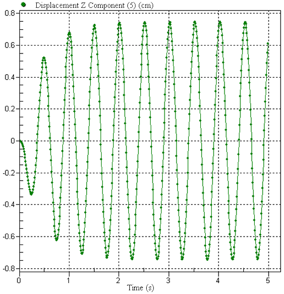
Figure 2: Displacement Plot of Mass.
An archive of the model and results (ground motion.ach) is located in the Models subfolder of the Autodesk Simulation installation directory.
This example can be solved using the methods from many vibration textbooks. This particular example is patterned after example 4-9 from Vierck, Robert K., Vibration Analysis, Harper & Row, 2nd Edition, pages 129-130.