To access advanced time step settings, go to: Setup  Model Setup Parameters Advanced Time-Step tab.
The information on this page applies to the following analysis types, except if indicated otherwise:
- Mechanical Event Simulation (MES)
- Static Stress with Nonlinear Material Models
- MES Riks Analysis
The Output interval field can be used to limit how often the results are written to the output files. A value of 1 will write the results after each time step, a value of 2 will write every other time step, and so on.
To start the analysis at a non-zero time, specify this time in the Starting time for event field. View the starting time as shifting the load curve and time step label shown in the results. However, the Starting time for event has no affect during a resume or restart analysis. In particular, the Starting time for event functions as follows:
- The analysis will run from the starting time to starting time + duration. The length of the analysis is still the user-entered duration.
- In the Results environment, time step number (load case) 0 corresponds to the starting time.
- As with any analysis, the load curves are interpolated based on this time.
- Although the analysis is starting at a nonzero time, the model is still beginning in a stress-free condition. What occurs prior to starting time is not calculated. The loads applied at the starting time will determine the stress state at the beginning of the analysis.
During the analysis, the processor will reduce the time step if convergence cannot be achieved or if distorted elements are encountered. To avoid this, activate the Use a constant time-step size check box. However, you may need to allow more iterations to achieve convergence (change the Maximum number of iterations field in the Equilibrium tab) and/or to recalculate the stiffness matrix more often than once per time-step (change the Number of allowable stiffness reformations per time step field on the Equilibrium tab).
You can control the situations that cause the time step to be decreased using the Decrease trigger: rate of convergence drop-down box.
- If the Avoided option is selected, the time step will never be reduced because of the convergence rate.
- If the Always accelerating option is selected, the time step will be reduced whenever the rate of convergence decelerates.
- If the Allow initial decrease option is selected, the analysis will allow for a local maximum and then will decrease the time step if the rate of convergence decelerates.
- If the Reacts to oscillations option is selected, the time step will be decreased if a cyclical or oscillatory pattern is detected during the iterations.
Finally, if the Automatic option is selected, the following will be chosen based on other model settings:
- The Allow initial decrease option will be used for models with any nonlinear material models and no contact.
- The Always accelerating option will be used for models containing only linear materials and no contact.
- Avoided will be used for models with surface-to-surface contact.
Two additional decrease trigger options are available:
- If the Decrease trigger: allow for non-monotonic convergence check box is activated, the time step will be reduced if the iteration tolerance is decreasing monotonically. This option is enabled by default.
- If the Decrease trigger: high solution tolerance check box is activated, the time step will be reduced if the iteration results in a solution tolerance greater than 1. This option is enabled by default.
The Time step change factor drop-down box controls the factor by which the time step is reduced whenever the analysis fails to converge. (Likewise, the time step increases by the Time step change factor when the model is converging and a larger time step can be used.) In particular, the current time step size DT is related to the time step level L as follows:
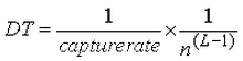
where n is the Time-step change factor. (Also see Setting Up and Performing the Analysis: Performing the Analysis: Performing A Nonlinear Analysis.)
You can also control the situations when the time step is increased after a solution is converged at the reduced time step:
- The value in the Increase trigger: number of convergent time-steps field controls how many monotonically convergent time steps must occur before the time step will be increased.
- The value in the Increase trigger: increment to number of convergent time-steps field controls how many additional time steps it will take before the time step is increased again, after it failed to converge at the increased time step.
The Time step reduction if there are distorted elements check box is activated by default. The time step size will be reduced if you obtain overly compressed or severely distorted elements during the simulation. When this option is disabled, an alternative method is used to help the solution to converge. Specifically, the integrity of the elements is maintained by the imposition of an artificial stiffness. While this alternative method does help the solution to converge, it also decreases the accuracy of the solution. Therefore, the default behavior is generally preferred.
If BOTH of the following statements are true, it may be appropriate to deactivate the Time step reduction if there are distorted elements checkbox:
- Time step reduction is not sufficient to produce solution convergence, and the log indicates that the time step is being reduced due to distorted elements.
- The elements that are becoming severely distorted are not of interest. This may be the case if there are concentrated (nodal) loads or constraints in non-critical regions, for example.