The information on this page applies to the following analysis types except where indicated:
Mechanical Event Simulation (MES)
Static Stress with Nonlinear Material Models
In a mechanical event simulation analysis and a static stress with nonlinear material analysis, a majority of the loads follow load curves. The load curves are defined in the Load Curves tab of the Analysis Parameters dialog. Any shape of curve can be entered here.
Select the Add next load curve or Add load curve button to add another load curve. You can have different loads follow different loading curves. For example, gravity may be constant throughout the analysis, so it is assigned to one load curve. A force may vary sinusoidally to simulate a rotating imbalance, so it is assigned to a different load curve.
The load curve is defined in the Data for Selected Load Curve section by a set of points that idealizes the real curve by a series of straight line segments. The first column is either time or a result (see details below), and the remaining columns adjust the loads assigned to the load curve, typically by multiplying the load. (Actuator elements and prescribed displacements use the load curve multiplier as the change in length or rotation, not as a multiplying factor.) The load curve is linearly interpolated as necessary to determine the multiplier at the corresponding time or result.
Use the Add Row button as necessary to define more points on the load curve, or the Delete Row button to remove the current row. The load curve data points need to be entered in ascending order by the time or result; use the Sort button if the data is not entered as such.
You can also import a load curve using the Import load curve button. First, create a text file in a Comma Separated File (.csv) format where each line of the text file corresponds to a row of the load curve, and a comma separates each value on the line for each column of the load curve. (The load curve's Index column is not included in the text file.)
- The destination load curve should have the same number of columns as the CSV file. For example, if using a CSV file with 4 columns for a results-based load curve, use the Add load curve and Add Column buttons as needed to create a blank load curve table with 4 columns.
- The values in the comma-separated file are imported using the active Display Units. Change the Display Units if necessary before importing the data. For example, a value of 3.14 is imported as 3.14 second if the Display Units are set seconds, and 3.14 minutes if the Display Units are minutes.
Time-Based Load Curves
When the load varies as a function of time, choose Time in the Data for Selected Load Curve section. The load curve then has two columns: Time and Multiplier 1. Enter the data points for the load curve directly into the Load Curve spreadsheet, or import the load curve (see above).
Note that the Time column of the load curve is converted based on the active Display Units.
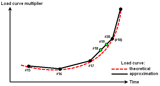
When approximating a higher order curve with a series of straight line segments, the spacing of the points in the load curve should be smaller than the smallest time step that will be encountered in the analysis. For example, imagine a runway crane that accelerates at a known rate. This is simulated by applying a prescribed displacement at the location of the wheels, where the displacement versus time is d = 0.5*a*t^2. If the load curve is calculated and entered at time steps t based on the capture rate, then the curve is followed precisely as long as the time steps are never reduced in the analysis. As soon as the time step is automatically reduced to converge on the solution, the load curve is interpolated. When this occurs, the prescribe displacement is not following the precise acceleration equation. See Figure 1.
|
|
|
Figure 1: Section of a Load Curve
Time steps #15, #16, and #17 follow the theoretical curve. If step #18 were able to converge, the load would still be on the theoretical curve (#18). But when the time step is reduced, steps #18 and #19 are interpolated, so this results in a slightly different load. In many cases, the difference is negligible (especially considering the approximations made by FEA in general). |
Result-Based Load Curves
Imagine magnetic contacts in a switch assembly. The force due to magnetic attraction is not a known function of time because the displacement of the contact (due to other loads in the analysis) versus time is unknown. The magnetic force varies depending on the separation between the parts. In this situation, define a load curve as a function of a result, and the analysis will vary the load appropriately throughout time.
Before accessing the Analysis Parameters dialog to define a result-based load curve, add probes to the model. The probes are the locations in the model whose results are used in the load curve. To add a probe, select a vertex or multiple vertices (Selection Select Vertices), right-click, and choose Add Nodal Probe. A dialog appears in which a description can be entered for the nodal probe objects. (See the page Loads and Constraints: Probes.)
To set the load curve to be based on a result, choose Lookup Value in the Data for Selected Load Curve. The load curve then starts with two columns: Lookup and Multiplier 1. (Addition columns can be added as described below.) The Lookup Value is defined with the Define/Edit Lookup Values button. Once defined, the lookup value can be set with the Lookup Value pull-down. The name of the lookup value will become the heading of the first column of the load curve spreadsheet.
- Prescribed displacements and actuator elements cannot use a results-based load curve.
- The first column of the lookup load curve - which contains the results of the lookup value equation - is not converted based on the active Display Units. The units for the lookup value and first column are based on the Model Units.
Define and Edit Lookup Values
Clicking the Define/Edit Lookup Value button will display the Define Lookup Value dialog which is where the lookup values are defined based on results at given locations. The functions on the Define Lookup Value dialog are as follows, listed in the order in which they are normally used.
- Click the Add button to define a new lookup value. The lookup value created must be a unique name but cannot contain any spaces. Time is also not an acceptable name to avoid confusion with the analysis time.
- Use the Lookup value name pull-down to view the input for any previously defined names. Once the input is displayed, any of the input can be changed, and it will be saved when switching to another lookup value or clicking the OK button to close the dialog.
- Click the Add Row button to add additional rows to the variable spreadsheet. The variables defined in the spreadsheet are used in the equation which defines what result is associated with the lookup value. Each variable added is automatically given the name V1, V2, and so on. The name of the variables can be changed to something more descriptive by clicking on the name in the spreadsheet.
- In the spreadsheet, select a probe and a result for each of the variables using the pull-downs. Only probes added to the model are available for the variable definition. The results that can be used at the probe are as follows:
- X Displacement
- Y Displacement
- Z Displacement
- X Velocity
- Y Velocity
- Z Velocity
- The Equation text box is where the variables described in the spreadsheet are combined to define the lookup value name. (Other lookup values cannot be included in the equation.) For example, if the result is as simple as the Y displacement of a node, the equation would be V1, where V1 is defined as the Y displacement at the relevant probe. If the lookup value name needs to be the average of three nodes, then the equation would be (V1+V2+V3)/3. The following operators can be used in the equation:
Operator Description (and)
Parentheses to group operations.
** or ^
Exponent function, or raises a number to a power. For example, V1^2 will give the square of the variable V1.
*
Multiplication.
/
Division.
+
Addition. -
Subtraction or negates a number, such as V1-V2, or -V1*5.
cos( )
Cosine of the value in parentheses. The value must be in radians.
sin( )
Sine of the value in parentheses. The value must be in radians.
tan( )
Tangent of the value in parentheses. The value must be in radians.
exp( )
Natural exponential function of the value in parentheses, or e raised to a power, such as e V1 .
log( )
Natural logarithm of the value in parentheses, or logarithm of the base e, often written in mathematics as ln( ).
abs( )
Absolute value of the value in parentheses.
sqrt( )
Square root of the value in parentheses.
acos( )
Inverse cosine function of the value in parentheses, or arc cosine.
asin( )
Inverse sine function of the value in parentheses, or arc sine.
atan( )
Inverse tangent function of the value in parentheses, or arc tangent.
cosh( )
Hyperbolic cosine of the value in parentheses.
sinh( )
Hyperbolic sine of the value in parentheses.
tanh( )
Hyperbolic tangent of the value in parentheses.
log10( )
Base 10 logarithm of the value in parentheses, often written in mathematics as log( ).
Condition Statements and Multiple Load Curve Multipliers
As described thus far, the lookup value selected for the load curve becomes the single value that is used to determine the multiplier for the load - just like time is the single value in a time-based load curve that is used to determine the load multiplier. There are situations in which multiple results or multiple lookup values are affecting the magnitude of the load. In these situations, the Condition text box is used in conjunction with multiple columns in the spreadsheet to determine which multiplier column is interpolated based on the selected lookup value.
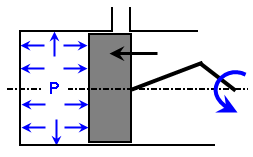
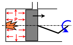
For example, imagine a 2-cycle engine, shown schematically in Figure 2. Note that the piston's position is the same in figure 2a as in figure 2b. However, the pressure in figure 2a is based on the supply pressure and the motion of the piston since the exhaust port became closed (compressing the gas), and the pressure in figure 2b is based on the combustion pressure and the motion of the piston since combustion (expanding the gas). Thus, the load curve cannot be based on the piston's position, but it can be based on the piston's position and velocity. This type of control is obtained by using the Condition text box. The format is as follows:
IF (Lookup Value test comparison; multiplier column if true; multiplier column if false)
where
- Lookup Value is an existing lookup value name, created and defined with the Define/Edit Lookup Values.
- test is one of the following conditional symbols:
Symbol Description >= or =>
Greater than or equal to
<= or =<
Less than or equal to
=
Equal to
>
Greater than
<
Less than
- comparison is a numerical value. It cannot be another lookup value. So to use a lookup value, such as Vel1>Vel2, define a new lookup value Vel3 = Vel1 - Vel2 and use the comparison test Vel3>0.
- multiplier column if true is a number that indicates which multiplier column to use from the load curve when the comparison test is true
- multiplier column if false is a number that indicates which multiplier column to use from the load curve when the comparison test is false
Note that the semi-colon character (;) is used to separate the three parts of the IF condition.
|
(a) The supply gases are compressed. |
(b) The combustion gases are expanding. |
|
Figure 2: Two-Cycle Piston
Although the position of the piston is the same in these two positions, the pressure P is different. |
|
Based on the result of the conditional test, the appropriate column of the load curve spreadsheet will be interpolated. Use the Add Column and Delete Column buttons to add or remove multiplier columns from the spreadsheet. If no condition statement is used (the Condition text box is blank), then only Multiplier 1 column will be used regardless of how many columns are entered into the spreadsheet.
- The condition equation can be nested so that and type operations can be included. For example, let's break down the statement IF(sep1<10;3;IF(vel>0;1;2)). If the result defined by the variable sep1 is less than 10, then use multiplier column 3 (true condition). If sep1 is not less than 10 (the false condition), then the multiplier column for the false condition is another test which needs evaluated - if the result defined by the variable vel is greater than 0, then use the multiplier in multiplier column 1; if the vel is not greater than 0, use multiplier column 2. To summarize,
- use multiplier column 3 if sep1 is less than 10.
- use multiplier column 1 if sep1 is greater than or equal to 10 and if vel is greater than 0.
- use multiplier column 2 if sep1 is greater than or equal to 10 and if vel is less than or equal to 0.
Example 1: Magnetic Forces
For the magnetic force example shown in Figure 3, imagine the following parameters:
- X = 0.5 inches in the rest position (before activating the magnets)
- F = 0.3125/(S^2) after activating the magnets, where S is the actual separation
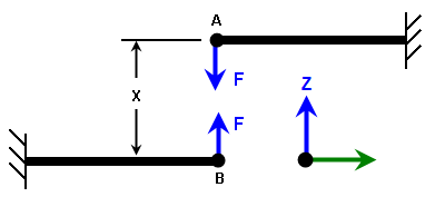
Figure 3: Magnetic Attraction Example
The steps specific to the setup the magnetic forces are as follows:
- Select the top node A (Selection Select Vertices) and apply a nodal force (right-click Add Nodal Force). Set the magnitude of the force to -1 and the direction to the Z direction. By using a unit force, the load curve multiplier will be the total magnetic force. Click the OK button to apply the force.
- With the node still selected, add a probe (right-click ). Enter a description of Top Node and click the OK button.
- Select the bottom node B (Selection Select Vertices) and apply a nodal force (right-click Add Nodal Force). Set the magnitude of the force to +1 and the direction to the Z direction. Click the OK button to apply the force.
- With the node still selected, add a probe (right-click Add Nodal Probe). Enter a description of Bottom Node and click the OK button.
- Access the Analysis Parameters dialog (Analysis: Parameters) and choose the radio button to set the load curve type to Lookup Value. The first column of the load curve spreadsheet changes from Time to Lookup Value.
- Define a new variable that represent the calculated separation between the two magnets. Click the Define/Edit Lookup Values button. This opens a new dialog. Click the Add button and enter the new variable name Separation. Click the OK button to complete the entry of the lookup value name and return to the Define Lookup Value dialog.
- The separation is an equation based on the displacement of two nodes, so click the Add Row button once to add a second variable, V2, to the spreadsheet.
- For the variable V1, select the probe Top Node and result of Z Displacement.
- For the variable V2, select the probe Bottom Node and result of Z Displacement.
- The equation for the calculated separation is then entered in the Equation text box. Type 0.5+V1-V2. Note that a positive displacement of the top node will increase the separation; hence V1 is added to the initial separation of 0.5. A positive displacement of the bottom node will decrease the separation; hence V2 is subtracted from the initial separation of 0.5.
- Click the OK button to close the Define Lookup Value dialog.
- Back on the main Analysis Parameters dialog, use the Lookup Value pull-down and choose Separation as the lookup value. The first column of the load curve spreadsheet changes from Lookup Value to Separation.
- Finally, evaluate the multiplier (the magnetic force in this setup) at various separations and enter them into the load curve spreadsheet. Although the force is infinite in theory when the separation is 0, the following load curve is more practical from an FEA perspective (where contact is required to prevent the parts from passing through each other, so the separation should not reach a magnitude of 0). Note the additional entries for separation greater than 0.5 (the initial separation). You want the load curve to cover all possible ranges of separation should the items vibrate or other loads cause them to be further apart than the initial separation.
Index Separation Multiplier 1 1
0 100 2
0.1
31.25
3
0.2
7.81
4
0.3
3.47
5
0.4
1.95
6
0.5
1.25
7
0.6
0.868
8
0.7
0.638
9
0.8
0.488
- Click the View Plot button to confirm the shape is hyperbolic as expected. It looks as if more data points are needed between 0 and 0.2 to produce a smoother curve.
Example 2: Two-Cycle Pistons
For the 2-Cycle piston shown in Figures 2 and 4, imagine the following (fictitious) parameters:
- X = -1.25 inch (X displacement of the piston when the exhaust port is fully blocked)
- Compression stroke = 1.5 inch (X0 = -1.5)
- Bore = 3 inch diameter
- V0 = 14.2 inch^3 = volume of trapped air when the exhaust port is closed
- Supply pressure = 10 psig
- Combustion pressure = 1000 psig
- Each phase is an isothermal process; the gas pressure can be calculated from the ideal gas law.
- Approximate the volume of the trapped air between the piston and the cylinder head from the distance the piston has moved from X0. The change in volume due to the expansion of the cylinder bore will be ignored in this discussion.
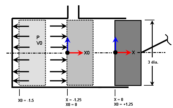
Figure 4: 2-Cycle Piston Example
The piston is shown in three positions. X=0 is the position the model is drawn, X0=0 is when the exhaust port becomes blocked, so the trapped gases have a volume of V0 and pressure P, and X0=-1.5 is the forward position of the piston.
Naturally, the pressures applied in the load curve can be more sophisticated than the ideal gas law to take compressibility and heat losses into account. Also, this write-up only includes the pressure on the cylinder head and blind side of the piston. Additional work is required to include the pressure on the sides of the cylinder walls and on the rod end of the piston; these pressures follow a different result-based load curve.
- Select the surfaces (Selection Select Surfaces) on the blind end of the piston and cylinder head and apply a unit pressure of 1 psi (right-click and Add Surface Pressure/Traction). Check the box Follows Displacement and click the OK button to apply the pressure.
- Ignoring the deflection of the cylinder head, the volume of the trapped air can be calculated solely from the position of the piston. Select a node on the piston (Selection Select Vertices), right-click, and choose Add: Nodal Probe. Enter a description of Piston and click OK to add the probe.
- Access the Analysis Parameters dialog (Analysis: Parameters) and choose the radio button to set the load curve type to Lookup Value. The first column of the load curve spreadsheet changes from Time to Lookup Value.
- Define a new variable that represent the position of the piston relative to the exhaust port, or the position X0 in Figure 4. Click the Define/Edit Lookup Values button. This opens a new dialog. Click the Add button and enter the new variable name X0. Click the OK button to complete the entry of the lookup value name and return to the Define Lookup Value dialog.
- For the variable V1, select the probe Piston and result of X Displacement.
- The equation for the piston position relative to the exhaust port X0 is then entered in the Equation text box. Type V1+1.25.
- Define a new variable that represent the velocity of the piston. Click the Add button and enter the new variable name Velocity. Click the OK button to complete the entry of the lookup value name and return to the Define Lookup Value dialog.
- For the variable V1, select the probe Piston and result of X Velocity. Note how the same probe is used for multiple lookup values. Also, the variable V1 in the lookup value X0 is completely independent of the variable V1 in the lookup variable Velocity.
- The equation for the piston velocity is simply the variable V1. Type V1 in the Equation text box and click the OK button to close the Define Lookup Value dialog.
- Back on the main Analysis Parameters dialog, use the Lookup Value pull-down and choose X0 as the lookup value. The first column of the load curve spreadsheet changes from Lookup Value to X0.
- A condition based on velocity is required in this analysis, as described previously. Enter the text IF(Velocity>0;1;2) in the Condition text box. When the velocity is positive (piston moving to the right), the combustion gases are expanding, and multiplier column 1 will be used. When the velocity is negative (piston moving to the left), the supply gases are being compressed, and multiplier column 2 will be used.
- Click the Add Column button to add a second multiplier column to the load curve spreadsheet.
- Finally, evaluate the multipliers (the pressure in this setup) at various positions of the piston and enter them into the load curve. Using the Ideal Gas Law, the pressure Pc for the compression stroke (-1.5<=X0<=0) can be calculated from the initial pressure Psupply and volume Vinitial as follows:
Pinitial*Vinitial = P*V
Psupply*V0 = P*(V0+X0*(pi/4)*Bore^2)
(10 psig + 14.7 psi)*(14.2 inch^3) = (Pc+14.7 psi)*(14.2 inch^3+7.0686*X0)
Pc = 350.74/(14.2+7.0686*X0) - 14.7
and for the expansion stroke, the gage pressure Pe can be calculated from
Pinitial*Vinitial = P*V
Pcombustion*(V0 - (stroke)*(pi/4)*Bore^2) = P*(V0+X0*(pi/4)*Bore^2)
(1000 psig + 14.7 psi)*(14.2 inch^3-10.60 inch^3) = (Pe+14.7 psi)*(14.2 inch^3+7.0686*X0)
Pe = 3652.92/(14.2+7.0686*X0) - 14.7
Index
X0
Multiplier 1
(gases expanding, Pe)
Multiplier 2
(gases compressing, Pc)
1
-1.75
1981
177
2
-1.5
1000
82.8
3
-1.25
666
50.7
4
-1.0
498
34.5
5
-0.5
328
18.2
6
0
243
10
7
0.1
10
10
8
10
10
10
Note the gradual change in pressure as the exhaust port is opened (0<X0<0.1). Also, the piston theoretically never displaces to positions -1.5<X0, but some lead way is necessary for round off and deflections of the system. Thus, the load curve is calculated for a stroke of -1.75.