Membrane elements are three- or four-node elements formulated in three-dimensional space. Membrane elements are used to model fabric-like objects such as tents or cots, or structures such as the roof of a sports stadium, in which the elements do not support or transmit a moment load.
Membrane elements model solids of a specified thickness which exhibit no stress normal to the thickness. The constitutive relations are modified to make the stress normal to the thickness zero. The highest surface number among the lines that define the element determines the surface number of that element.
Membrane elements, by definition, cannot have rotational degrees of freedom (DOFs), even if you released these DOFs when you apply the boundary conditions. You can apply translational DOFs as needed. However, only in-plane stiffnesses are formulated. Very small out-of-plane stiffnesses are applied to provide stability. Consequently, only in-plane (membrane) loads are admissible. Temperature-dependent, orthotropic material properties can be defined and incompatible displacement modes can be included. Stress output is provided at the nodes.
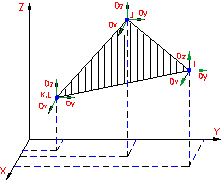
Figure 1: Membrane Element (Triangular)
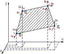
Figure 2: Membrane Element (Quadrilateral)
When to Use Membrane Elements
- The thickness of the element is very small relative to the length or width.
- The element has no stress in the direction normal to the thickness.
- The element does not carry or transmit any moments.
Membrane Element Parameters
When using membrane elements, you must define the thickness of the part in the Thickness field of the Element Definition dialog box. The element is considered to be drawn at the midplane of the membrane element. Therefore, half of the entered value for thickness are considered on top of the element while the other half are below the midplane. Enter a value for the thickness to run the analysis.
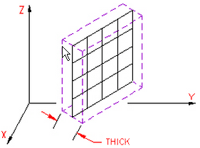
Figure 3: Thickness of a Membrane Element
Next you must specify the material model for this part in the Material Model drop-down Menu. If the material properties in all directions are identical, select the Isotropic option. If the material properties vary along three orthogonal axes or if properties change with temperature, select the Orthotropic option.
When the orthotropic material model is used for membrane elements, three material axes are defined. These are the n, s and t axes. By default, the n axis is parallel to the ij edge of the element. The t axis is normal to the element and points away from the Element Normal Coordinate (specified on the Orientation tab). The s axis is in the plane of the element and is 90 degrees from the n axis. (It follows the right-hand rule about the t axis, or s=txn.) To rotate the material axis, specify an angle in the Material Axis Rotation Angle field. The n axis is rotated by this angle about the t axis (right-hand rule).
If you are performing a thermal stress analysis on this part, specify the temperature at which the elements in this part experiences no thermally induced stresses in the Stress Free Reference Temperature field. Element based loads associated with constraint of thermal growth are calculated using the average of the temperatures specified on the nodal point data lines. The reference temperature is used to calculate the temperature change. Thermal loading may be used to achieve other types of member loadings. For these cases, an equivalent temperature change (dT) is used.
The last parameter that can be defined is the compatibility. This is done in the Compatibility drop-down menu. If the Not Enforced option is selected, gaps or overlaps are allowed along inter-element boundaries. These elements are formulated using an assumed linear stress field. These elements are most effective as low aspect ratio rectangles. If the Enforced option is selected, overlaps or discontinuities are not allowed along inter-element boundaries. These elements are formulated using an assumed linear displacement field. These elements can overestimate the stiffness of the structure. In general, a greater mesh density in the direction of the strain gradient is required to achieve the same level of accuracy as elements for which the Not Enforced option is selected. See Incompatible Displacement Modes for more information.
Control Orientation of Membrane Elements
An element normal point is also used to control the orientation of a membrane element. This point is defined using the X Coordinate, Y Coordinate, and Z Coordinate fields in the Element Normal section. Each element has a local set of axes labeled 1, 2 and 3. The local 1 axis goes through the jk side of the element. The local 3 axis is perpendicular to the membrane element and points away from the element normal point. The local 2 axis is the cross product of the local 1 and 3 axes. See Figure 4.

|
| Figure 4: Determining the Element Normal The edge-on view of the membrane element is shown. |
For a general FEA analysis, you can ignore the element orientation. The ability to orient elements is useful for elements with orthotropic material models and for easily interpreting stresses in local element coordinate systems. This is done in the Orientation tab of the Element Definition dialog box. The Method drop-down menu contains three options that can be used to specify which side of the element is the ij side. If the Default option is selected, the side of an element with the highest surface number is chosen as the ij side. If the Orient I Node option is selected, a coordinate must be defined in the X Coordinate, Y Coordinate, and Z Coordinate fields. The node on an element that is closest to this point is designated as the i node. The j node is the next node on the element following the right-hand rule about the element's normal axis (+3). If the Orient IJ Side option is selected, a coordinate must be defined in the X Coordinate, Y Coordinate, and Z Coordinate fields in the Nodal Order section. The side of an element that is closest to this point is designated as the ij side. The i and j nodes are assigned so that the j node can be reached by following the right-hand rule about the element's normal axis (+3) along the element from the i node.
To Use Membrane Elements
- Be sure that a unit system is defined.
- Be sure that the model is using a structural analysis type.
- If you are going to apply a pressure load along the edge to this element, the edge where the load will be applied must be the highest surface number on the element.
- Right-click the Element Type heading for the part that you want to be membrane elements.
- Select the Membrane command.
- Right-click the Element Definition heading.
- Select the Edit Element Definition command.
- In the General tab of the Element Definition dialog, select a material model in the Material Model drop-down box. Select the Isotropic if the material properties are independent of direction. Select the Orthotropic option if the material properties are dependent of direction.
- Enter the thickness of the membrane elements in the Thickness field. This is required information and must be entered to run the model.
- If you are performing a thermal stress analysis, enter a temperature value in the Stress Free Reference Temperature field. The difference between this value and the applied temperatures will be used to calculate the stress.
- For an orthotropic material model, if the material axes do not lie on the global XYZ axes, enter the rotation angle value in the Material Axis Rotation Angle field. This angle is measured counterclockwise from the global Y axis to the material axis in degrees.
- To define a local set of axes for the element (useful for orthotropic material models), select either the Orient I Node or Orient IJ Side options in the Method drop-down box and define a point in the X Coordinate, Y Coordinate and Z Coordinate fields in the Nodal Order section. If the Orient I Node option is chosen, the corner of each element closest to the point will be the I node. If the Orient IJ Side option is chosen, the side of each element closest to the point will be the IJ side.
- Press the OK button.