Critical Buckling Load

Critical buckling load analysis (also known as Eigenvalue buckling analysis) examines the geometric stability of models under primarily axial load. Buckling can be catastrophic if it occurs in the normal use of most products. Once the geometry starts to deform, it can no longer withstand even a fraction of the initially applied force.

The element types available for critical buckling are beams, plates, and bricks (and their variations). The element chosen can affect the type of buckling multiplier calculated. For example, beam elements are only a line with the cross-section represented mathematically; beams can only calculate a global buckling. Plate and brick elements can calculate localize buckling since the cross-section is modeled with elements. See Figure 1.


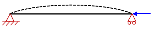
(a) Beam elements give a global buckling shape and load multiplier.
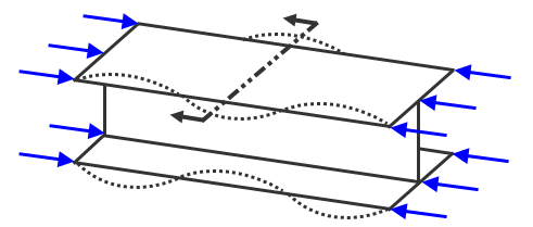	cross section
(b) Plate and brick elements can give global and local effects. In this example, the flange of the beam buckles locally which may be at a critical load less than the load to cause global buckling.
Figure 1: Eccentric Load on Column or Bar

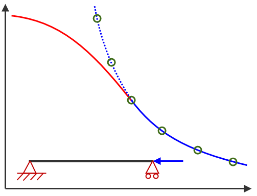
Since the critical buckling is calculated by solving an eigenvalue problem (like a modal analysis), the results are suitable for thin and slender structures (like Euler columns). No corrections are incorporated for short columns, thick plates (compared to the length and width of the plate), or the yield strength of the material. See Figure 2. Also, it is a linear analysis. There are no stiffness changes due to the deflection and therefore no large deflection effects such as P-delta (load-deflection) effects. Consequently, the critical load and buckling mode shape can be determined, but what happens after buckling is not available. (Perform nonlinear analysis if post-buckling results are needed.)

Critical Load

Euler Equation Johnson correction calculated results	Slenderness Ratio
Figure 2: Eccentric Load on Column or Bar

Use buckling analysis to determine if a specified set of loads cause buckling and to find the shape of the buckling mode. You can then design supports or stiffeners to prevent local buckling. It is useful in situations where a part or assembly is subjected to an axial load or when a model undergoes edge compression.

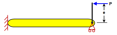
Loads that do not cause compression do not affect the buckling calculation. It is important to note that when calculating the critical buckling load for beam elements, only the axial component of the loads are considered. For example, imagine an offset load on the end of a bar (see Figure 3(a)). It can be represented as an axial load and moment on the end of a beam model (Figure 3(b)). Since the moment does not create axial stress in the beam elements, the offset load in this analysis produces the same result as a pure axial load. (The moment creates bending stresses; the theoretical compression on one side of the beam element does not affect the buckling calculation.)

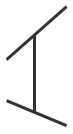
(a) Physical model of a bar with a load P offset from the centerline by a distance e.

(b) Beam model created in FEA. The load eccentricity results in a moment applied to the node. Due to the nature of beam elements and critical buckling, the moment does not affect the results. The wrong element type is used in this example.

Figure 3: Eccentric Load on Column or Bar

The calculated buckling load multipliers are shown in the Results environment, in the log file, and in the summary file. The buckling load multiplier indicates when the model will buckle. Multiply all the applied loads on the model by the buckling load multiplier, and it is the theoretical load that causes buckling. Real parts tend to buckle at lower loads than the theoretical value due to imperfections in real-life manufacturing (initial curvature, eccentrically applied loads, and so on). Small deviations can have enormous effects on the critical load in reality.

If the buckling load multiplier is negative, it indicates that reversing the applied loads (and scaling by the multiplier) cause the model to buckle. For example, a pressure of 1000 Pa is applied to the model. But the pressure puts it into tension. A buckling multiplier of -0.75 indicates the part will buckle with a 750-Pa compression load.

Include constant loads

Critical buckling scales all applied loads by the calculated buckling multiplier. In some situations, you might want to scale the live loads (like pressure) while other loads (like gravity) are not scaled. Use the following procedure if the constant loads are significant and must be included.

Estimate what the buckling multiplier will be, either from experience, doing a hand calculation, or running the analysis. Call it the last buckling multiplier.
Change the constant loads to the quantity (constant load/last buckling multiplier) and leave the live loads at their rated value.
Run the buckling analysis.
If the result of the new buckling calculation gives the same buckling multiplier, then the solution is okay. The constant loads at the buckling result is (constant load/last buckling multiplier)*(new buckling multiplier) = constant load, and the variable load that causes buckling is (variable load)*(new buckling multiplier).
If the result of the new buckling calculation gives a different buckling multiplier, replace the last buckling multiplier with the new value. Repeat steps 2 through 5.

Since critical buckling is an eigenvalue solution, the displacement results show the buckling mode shape. The magnitude of the displacements is meaningless. Likewise, there are no stress or strain results from a critical buckling analysis.