Overview of Process
When the conduction coefficient is a function of temperature (orthotropic material model) or when radiation is applied to the model, multiple iterations must be performed to solve the steady-state heat transfer analysis problems. For example, without knowing the temperatures, the thermal conductivity is not known, but the temperatures cannot be calculated without the thermal conductivity. Thus, an iterative approach is required.
In addition to using temperature-dependent conductivity and radiation for straight forward purposes, use these effects to calculate body-to-body radiation and convection as a function of temperature as described in the following section.
On each iteration of the steady-state solver, the temperature-dependent conduction coefficients and the radiation heat transfer rates are estimated based on the prior estimate of the nodal temperatures, (T i cur). On the first iteration, the initial temperatures are given by either the values applied to the nodes individually (right-click a node and select the Add: Temperature command) or globally (Default nodal temperature in the Options tab of the Analysis Parameters screen). When initial temperature values are specified for nodes in the FEA Editor environment, those values over-ride the default values. The model is then analyzed. The resulting temperatures (Ti new ) are compared to the prior estimate of the nodal temperatures. If the difference between the prior and resulting temperatures is acceptable, as defined below, then the analysis iterations stop. If the difference is not acceptable, then the thermal conductivity and radiation heat rates are recalculated based on the new assumed nodal temperature estimates and the problem is solved again. This process is shown in figure 1.
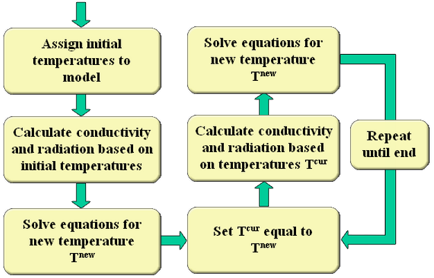
Figure 1: Nonlinear Solution Process
In reality, the temperatures used to calculate the conductivity or radiation on the next iteration (T cur )are calculated as [(1-A)(T i old )+(A)(T i new )] or as the equivalent [T i old +A(T i new -T i old )] where A is the relaxation parameter (defined in the Relaxation parameter field in the Advanced tab of the Analysis Parameters screen) and T i old is the temperature calculated on the previous iteration. An A value of 1 is normally recommended. The assumed temperatures for the next iteration are the resulting temperatures (T i new ) from the iteration just performed. Values between 0 and 1 are used when it is desired to update the temperatures T cur by a smaller amount to damp out possible overshoot oscillations. Since a value of 0 would cause the temperatures not to be updated, use a nonzero relaxation parameter. A relaxation parameter not equal to one is needed when the nodal temperatures cycle between successive iterations instead of converging smoothly.
The new assumed temperatures are used to update the conduction coefficients and recalculate the radiation equations and the process is repeated.
Conduction as a function of temperature
If you use an orthotropic material model, then you can specify conduction as a function of temperature. You supply a set of temperature values corresponding to conduction values. The orthotropic properties must be given in ascending temperature order. The range of temperatures encountered in the solution must not exceed the upper or lower temperature bound for which material properties are provided. Conduction coefficients are calculated by linear interpolating between the temperature values supplied.
The default value for the initial temperature is 0. If unchanged, the minimum temperature specified to determine the conduction coefficients must be less than or equal to 0. The initial temperatures are used to calculate the initial conduction coefficients. The nonlinear option described previously must be used to iterate on the temperatures to update the conduction coefficients.
Radiation
The heat flux (heat transfer/time/area) experienced by a surface subjected to radiation is described by the following equations:
where
- q = heat flux
- F rad = radiation factor, which includes absorptivity, emissivity and view factor effects
- σ = Stefan-Boltzmann constant
- X= the Radiation multiplier entered on the Analysis Parameters screen.
- T s = calculated surface temperature, units must be in absolute temperature (Rankine or Kelvin)
- T rad = ambient temperature, units must in absolute temperature (Rankine or Kelvin).
Being a surface based load, the radiation parameters F rad and Trad are specified on the Radiation tab of the Surface Properties screen. The model temperatures can be entered in degrees F or degrees C. They are converted to absolute temperatures by the input on the Radiation tab of the Analysis Parameters screen. The Stefan-Boltzmann constant is also specified on this screen.
The quantity (T s 4 -T rad 4 ) can be re-written as (T s 2 +T rad 2 )(T s +T rad )(T s -T rad ). If the quantity (T s 2 +T rad 2 )(T s +T rad ) is assumed constant, then a linear solution algorithm can be used. The nonlinear run time option substitutes T i old for Ts in the constant portion of the equation and iterates as described above. The relaxation parameter (A) may need to be reduced if the solution oscillates during the iteration process.
Body-to-body radiation
The type of radiation discussed previously is valid for a part that radiates to the ambient surroundings. In reality, often parts transfer heat through radiation with other surfaces on the same part and other parts. Right-click in the display area and select the Body-to-Body Radiation command or select Setup Thermal LoadsBody-to-Body Radiation. You can place the surfaces that will transfer heat with each other through radiation into separate enclosures. You can define the emissivities of these surfaces as constant values or temperature dependent values. See Body-to-Body Radiation for more details.
In some cases, body-to-body radiation can be emulated using temperature-dependent conduction as shown in the following figure:
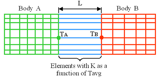
Figure 2: Body to Body Radiation
The requirements for this approximation to be accurate are as follows:
- The view factor between the bodies must be close to 1.
- The heat flux out of the system is negligible; that is, there is no radiation to the environment.
- The surface area of each body is equal.
- The expected temperatures of the surfaces are known either from hand calculations, experimentation, or previous analysis (multiple iterations).
The heat exchanged between two bodies which see each other and nothing else can be written based on the surface resistance and space resistance of the bodies as
Where T A and T B are the temperatures of surfaces A and B (in absolute temperatures), ε A and ε B are the emissivities of surfaces A and B, and VF AB is the view factor between the two surfaces.
The heat flow due to conduction between the two bodies is
Since the heat flow due to radiation must equal the heat flow by conduction, equating the above two equations and expanding![]() as follows
as follows
leads to the solution
using absolute temperatures.
One layer of elements is constructed in a new part between the two bodies. The material model is set to orthotropic so that the material properties are temperature dependent. The conductivity is calculated at estimated surface temperatures T A and T B (in absolute temperature) using the above equation. The calculated conductivity is entered in the material properties at a temperature of Taverage=0.5(T A +T B ) (in either absolute temperature or temperature, as set in the Units Definition dialog). Additional data points are entered by evaluating T average and K at other values of T A and T B . Be sure to include a range of temperatures T average in the material properties to that the calculated temperature is not outside of the range of material properties.
- Use only one element across the span L for the body to body radiation approximation. A mesh in the direction L must not be used.
- Different combinations of T A and T B can lead to different conductivities, K. The same temperature T average , the K to enter should be an average of all conductivities resulting for a given temperature T average .
Thermal loads as a function of temperature
Convection and heat generation loads can vary with temperature during a steady-state heat transfer analysis. To apply a temperature-dependent convection load, go to the Surface Properties screen and activate the Temperature Dependent Convection Coefficient checkbox in the Convection tab. You can then define a convection coefficient versus temperature curve that controls the heat flow due to convection through that surface. To apply a temperature-dependent heat generation load, go to the Element Definition and activate the Temperature Dependent checkbox in the Loading tab. You can then define a heat generation rate versus temperature curve that controls the heat generation through this part.