Average Element Thickness
The 11th user material constant defines the average element thickness used with energy-based degradation. For two-dimensional elements this value is ignored. For three-dimensional (solid) elements this is the average thickness of solid elements associated with the material, where the thickness is defined as the interlaminar dimension of the element.
Recall from Appendix A.5 that the final effective strain used in the energy-based degradation calculations is given by

In the above, Le is the representative element length as defined by Abaqus. In the case of three-dimensional elements (i.e. bricks and continuum shell) the element length is the cubed root of the volume. In the case of two-dimensional elements (i.e. shell and plane stress elements) the element length is the square root of the area.
For two-dimensional elements, the element thickness is ignored. The representative element length provides a measure of the in-plane area of the element, which gives us a meaningful measure to associate with a composite ply. However, for layered solid elements the representative element length is not associated with a measure for a single ply. To accommodate the use of solid elements and allow them to be used and compared against results for two-dimensional elements, the representative element length must be modified to provide a useful measure of the element length in the plane of a ply.
Composite fractures almost always occur in the plane of the lamina. Therefore, it is more accurate to neglect the through thickness size of the element. This is done by using the average element thickness constant supplied in the user material definition. The representative element length is then calculated as follows:

where Ve is the volume of the element, and te is the average thickness of the element. The element length defined in the equation above provides an accurate measure of the in-plane area of a solid element, and will collapse to the exact measure provided by Abaqus for two-dimensional elements when the thickness of a solid element is constant.
Degradation Time Period
In Abaqus/Explicit analyses which use instantaneous degradation, degrading the material properties instantly can have adverse effects on the response of the structure. Local material responses with large rates of change in stiffness can generate shockwaves in the material that prematurely initiate damage in adjacent elements. To mitigate this effect, we specify a time period over which to degrade material properties via user material constant 11. This value must be greater than or equal to zero. Larger time periods will result in smaller rates of change in stiffness.
When a failure is initiated the material properties are not automatically reduced to the next material state. The material stiffness is updated based on the following equation:
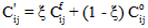
where  and
and  are the material stiffnesses at the next material state and previous state respectively, and
  is the updated (intermediate) material stiffness.
  is defined as:

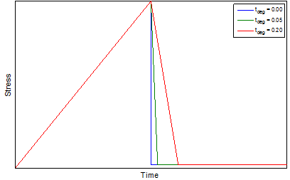
where ti, tf, and tdeg, are the current time, time at failure initiation, and the degradation time period (user material constant 11) respectively. The image below depicts the local material response as a function of time for different values of the time degradation period (constant strain after failure initiation).
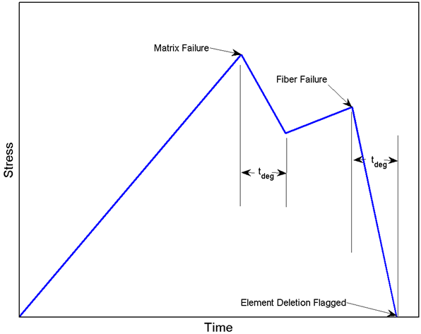
See the plot below for an idealized example of the stress at an integration point with respect to time.