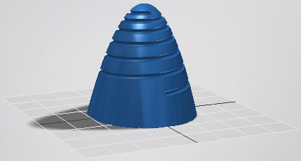
Use equation curves to model complex geometry such as gear tooth profiles, variable pitch threads, or sweep paths for hydraulic pumps. To generate an equation curve, specify the equations to define the curve and a range to evaluate the equations.
- On the ribbon, click 3D Model tab
 Sketch panel
  Create 3D Sketch
  . If a 2D sketch is active, right-click, and then select Finish Sketch to close the 2D environment.
 - On the ribbon, click 3D Sketch tab
 Create Panel
  Equation Curve to display the mini-toolbar.
 - Select Cartesian, Cylindrical, or Spherical to specify the coordinate system.
- Enter equations for x, y, z, or r, θ, z or r, ϕ, θ depending on the coordinate system selected.
- Enter the minimum and maximum values for t in the tmin and tmax fields.
- Click OK to create the curve and exit the command. Click Apply to create the curve and remain in the Equation Curve command.
- Add dimensions or constraints between the curve and other sketch geometry.
 Show Me how to create and use equation curves
Example Equation Format
This table shows examples of the formatting required to use certain operators and functions.
| Cartesian | Cylindrical | Spherical | |
|---|---|---|---|
|
Addition/Subtraction |
x(t): 1 mm * t + 1 mm y(t): 1 mm * t - 1 mm z(t): 1 mm * t - 1 mm |
r(t): 1 mm * t + 1 mm θ(t): 1 rad * t + 1 rad z(t): 1 mm * t - 2 mm |
r(t): 1 mm * t + 1 mm ϕ(t): 1 rad * t + 1 rad θ(t): 1 rad + t - 1 rad |
|
Multiplication/Division |
x(t):2 mm * t y(t):2 mm / t z(t): 2 mm / t |
r(t): 3 mm * t θ(t): 2 rad * t z(t): 2 mm * t / 2 |
r(t): 3 mm *t ϕ(t): 2 rad * t θ(t): 2 rad / 2 |
|
Exponents |
x(t): (t ^ 2) * 1 mm y(t): 1 mm * pow(t;2) z(t): 1 mm * pow(t;2) |
r(t): 1 mm * (t ^ 2) θ(t): 1 rad * pow(t;2) z(t): 1 mm * (t ^ (1/2)) |
r(t): 1 mm * (t ^ 2) ϕ(t): 1 rad * pow(t;2) θ(t): 1 rad * (t ^ (1/2)) |
|
Trig Functions |
x(t): 1 mm * sin(1 rad * t) + 1 mm * cos(1 rad * t) y(t): 1 mm * tan(1 rad * t) z(t): 1 mm * tan(1 rad * t) |
r(t): 1 mm * cos(1 rad * t) θ(t): 1 rad * sin(1 rad * t) z(t): 1 mm * tan (1 rad * t) |
r(t): 1 mm * cos(1 rad * t) ϕ(t): 1 rad * sin(1 rad * t) θ(t): 1 rad * tan(1 rad * t) |
|
Inverse Trig Functions |
x(t): 1 mm * asin(t) / 1 rad + 1 mm * asin(t) / 1 rad y(t): 1 mm * atan(t) / 1 rad z(t): 1 mm * atan(t) / 1 rad |
r(t): 1 mm * acos(t) / 1 rad θ(t): asin(t) z(t): 1 mm * atan(t) / 1 rad |
r(t): 1 mm * acos(t) / 1 rad ϕ(t): asin(t) θ(t): atan(t) |
|
Hyperbolic |
x(t): 1 mm * sinh(1 rad * t) + 1 mm * cosh(1 rad * t) y(t): 1 mm * tanh(1 rad * t) z(t): 1 mm * tanh(1 rad * t) |
r(t): 1 mm * cosh(1 rad * t) θ(t): 1 rad * sinh(1 rad * t) z(t): 1 mm * tanh(1 rad * t) |
r(t): 1 mm * cosh(1 rad * t) θ(t): 1 rad * sinh(1 rad * t) ϕ(t): 1 rad * tanh(1 rad * t) |
|
Log |
x(t): 1 mm * ln(t) y(t): 1 mm * log(t) z(t): 1 mm * log(t) |
r(t): 1 mm * log(t) θ(t): 1 rad * ln(t) z(t): 1 mm * ln(t) |
r(t): 1 mm * log(t) ϕ(t): 1 rad * ln(t) θ(t): 1 rad * ln(t) |
Edit 3D equation curves
Edit the equation to modify the curve. Use dimensions and constraints to control the position of the curve.
In an active 3D sketch, use one or more of these methods to edit an equation curve.
- Right-click the curve in the graphics window or the browser then select Edit Equation Curve to display the mini-toolbar. You can modify the equations, change the coordinate system, or edit the range.
- Add constraints to control relationships between the curve and other geometry. Equation curves support coincident, tangent, perpendicular, and fix constraints.
- Add a dimension between the endpoint of the curve and other geometry.
- Right-click on the curve and select Display Curvature to analyze the curvature of the equation curve.