Moldflow's fiber orientation models

Moldflow's fiber orientation models are based on the Folgar-Tucker orientation equation.

The Folgar-Tucker orientation equation is used for fiber orientation calculations on 3D meshes. The governing equation is:

Note the following:

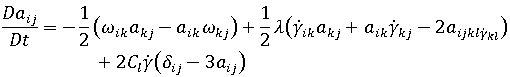
• is the fiber orientation tensor.
• is the vorticity tensor, and is the deformation rate tensor.
• is the fiber interaction coefficient, a scalar phenomenological parameter, the value of which is determined by fitting to experimental results. This term is added to the original Jeffery form to account for fiber-fiber interactions.

This fiber orientation model is further revised for calculations on Midplane and Dual Domain meshes. An extra term called a thickness moment of interaction coefficient () has been introduced into the model:

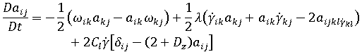
The following assumptions and considerations apply for this revised model:

• The Folgar-Tucker model gives acceptable accuracy for the prediction of fiber orientation in concentrated suspensions.

• Hybrid closure is used, as its form is simple and has good dynamic behavior.

Note the following:

• Setting = 0.0 sets the model back to the Jeffery form. affects the orientation tensor. If =0, fibers do not interact with each other; and if the value of becomes very large, fibers become less aligned.
• The magnitude of the term sets the significance of the randomizing effect in the out-of-plane direction due to the fiber interaction.
• Setting = 1.0 gives the Folgar-Tucker orientation model for the 3D problem. Setting = 0.0 gives the Folgar-Tucker orientation model for the 2D problem.

However, for injection molding situations, the flow hydrodynamics cause the fibers to lie mainly in the flow plane. Their ability to rotate out-of-plane is severely limited. This mechanism predicts that the randomizing effect of fiber orientation is much smaller in the out-of-plane direction than in the in-plane direction, hence a small value.

• Decreasing this parameter:
  • decreases the out-of-plane orientation.
  • increases the thickness of the core layer.
• The simulation treats the problem as being symmetric about the midplane.

Empirical versus scaled-volume fraction expression

The experimental work of Bay suggests that the interaction model of Folgar and Tucker does apply to injection molding problems. However, how does one know which value to apply in fiber orientation modeling?

Experiments by Folgar and Tucker indicated that depends on the fiber volume fraction and aspect ratio, but the form of the dependence was unclear.

The flow in a film-gated strip is mainly simple shear. The shell layer (covering 40-90% to the walls from the midplane) should take on the steady-state value for simple shear. This situation would offer a ready way of examining this dependence.

Bay's shell layer orientation results show that the orientation is very sensitive to fiber concentration, suggesting that an empirical relation for the interaction coefficient could be developed. Also, Bay's measurements support the proposal of making the fibers diffuse at a rate proportional to the strain rate.

From Bay's thesis, an expression was presented to provide an empirical relationship for the dependence of the interaction coefficient on some fiber details. The expression is a simple exponential term. The data comes from the shell layers of injection molded strips of different materials (PC, PBT, PA66) at 6-7 glass levels for each material. The cases may all be considered concentrated suspensions.

Revised empirical expressions

Based on the shell layer orientation results, the applicability of the default value from the Bay expression across the range of glass contents has been reviewed.

At the = 1.0 condition (Folgar-Tucker model form), the orientation is over-predicted for all glass contents of both materials. The level of over-prediction reduces as the glass content increases. See the figure below.

A series of Fiber Fill+Pack analysis validation procedures were performed using both an end gated strip and a centrally gated disk. A more detailed consideration of the shell layer orientation of the strip for two materials (PA66 and PBT) and at different glass levels was undertaken and the results compared with Bay's experimental orientation data. The orientation levels were typically 0.8.

Revised empirical expressions for versus the scaled volume fraction cL / d at = 0.01 and 1.0 were derived, using the packing phase results.

A more complex procedure applies for intermediate values.

The figure below shows the error in shell layer orientation prediction for both materials at different glass levels for these cases:

• = 0 (the Jeffery model).
• Bay empirical expression for with = 1.0 (the Folgar-Tucker model).
• For typical injection-molded parts (part thickness <; 2.5 mm), the revised model with a low value, such as = 0.01 as a default, as proposed in the past, is shown in the graph below.
  
  
  

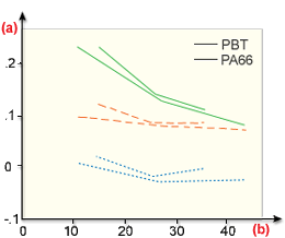
  Revised model with a low value

  .

  (a) Error; (b) % glass (weight);  = 0.0 (Jeffery Model);  Bay  ( =1.0);  Moldflow  Model (= 0.01)

• For thick parts (thickness > 2.5 mm), the revised model with = 1.0 is used. The value of has been shown to increase monotonically with part thicknesses. This increasing trend is consistent with the expectation that out-of-plane fiber orientation would increase with increasing part thickness.

The following observations can be made:

• The Jeffery and Folgar-Tucker models tend to lead to an over-prediction in the orientation estimates.
• The low model case results in substantially reduced error levels for thin parts (thickness < 2.5 mm).
• The default Bay model with low value provides orientation estimates that lie within the confidence band of the Bay experimental data, for all but the high glass levels.
• The revised model offers a substantially improved orientation prediction over the other model cases, for both materials and across all glass levels considered.

Summary of − combinations

The valid data range for the coefficient of interaction, , is 0-1.0; however, we have found that using values greater than 0.1 does not improve the predictions compared to experimental results.

The valid data range for the thickness moment of the interaction coefficient, , is 0.0001-1.0.

The interaction coefficient and thickness moment combinations which are allowed with this software release are summarized in the following table:

Coefficient of Interaction,	Thickness Moment of the Interaction Coefficient,	Comments
0	0.0001–1.0	Jeffery Model; dilute suspension ineffective Also set for volume fraction or fiber length set to zero
0 < <= 0.1	1.0	Folgar-Tucker Model
default	<= 1.0, (default = 1.0)	derived from empirical expression, according to scaled volume fraction ( cL / d ) using terms in mechanical properties and if d = 0 execution is aborted if cL / d = 0, then = 0. if 0 < cL / d < 1.0, then = 0.003 if cL / d > 1, then is calculated empirically Basically insensitive where < 0.01
User Set (0–0.1)	<= 1.0 (default = 1.0)	Other implementation allowed

Analysis scheme overview for fiber orientation

During the molding process, fiber orientation at a point is controlled by the fluid motion in two different manners: flow-deduced orientation (kinematic term) and flow-convected orientation (advection term).

For the kinematic term, the prediction accuracy depends upon the accuracy of the velocity gradient calculated.

For the advection term, its accuracy is dependent on the calculation of the orientation gradient. Like velocity, the representation of the orientation tensor is also coordinate system dependent. All numerical schemes suitable for the calculation of velocity gradients can be used to calculate the orientation gradient. In the fiber orientation software, the same element system is used to represent the velocity and orientation fields, consequently the same scheme is used to calculate the velocity and orientation gradients.

An outline of the overall fiber orientation scheme is now described. The fiber orientation prediction is coupled with the mold filling simulation.

First, the algorithm initializes for the filling and fiber orientation calculations.

The following loop is then repeated for the analysis until all elements are frozen:

• Determine time step for the Fill+Pack analysis.
• Advance the flow front.
• Calculate the pressure and velocity fields and the strain tensor.
• Calculate the stable time step for the advection term.
• Repeat time step until .
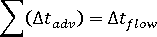• For each grid point in each element:
  • calculate the advection fiber orientation term until .
  • calculate kinematic fiber orientation term.
  • calculate time step , for kinematic term.
  • calculate new fiber orientation during time step .
• Return to the beginning of the loop.