Buckling analysis (Concept)

Whilst the full non-linear incremental/iterative method of following the response of a structure is completely general and relatively precise, it can also involve a great deal of computational effort.

Because of the fundamental importance of buckling, and its design implications, a simplified method that provides an approximation to the critical load level at which buckling can be expected to occur, will clearly be valuable. It turns out that such a method can be devised provided we assume that the prebuckling response is linear and that the effect of prebuckling displacements is negligible. The method, which we call buckling analysis, is also referred to as initial stability or classical bifurcation analysis.

The following sections describe the Generalized buckling analysis method and then the two specific methods used by the analysis.

Generalized Buckling Analysis

In buckling analysis, the aim is to determine the critical buckling load for some known distribution {P} of applied loading. By definition then, we can write:

where

is the critical level of the applied load distribution,
is an arbitrary level of the same load distribution (reference load), and
is a scalar multiplier.

With these definitions, buckling occurs when the load multiplier _{reaches a critical value . The starting point in buckling analysis is the assumption that each coefficient of the stiffness matrix varies linearly with the applied load. As described above, we can think of the applied load as some parameter (say ) multiplied by a constant vector of forces .}

Given two known states of the structure, (

and

), and our assumption of linearity, the stiffness matrix at any given equilibrium configuration,

, is given by:

If we define the fraction term as

, and the change in stiffness from

, then:

At a buckling point, there are two equilibrium configurations, {U} and

, both at the same load level.

This is illustrated in the Figures below, which shows the equilibrium configurations for the two basic types of buckling (these are discussed in more detail later).

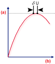
Limit point

(a) load, (b) Deflection

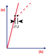
Bifurcation point

(a) load, (b) Deflection

Using the basic equation from linear analysis,

, we can therefore write:

where {U} are the displacements corresponding to loads {P], and

denotes the infinitesimal) displacements between the two equilibrium configurations. Subtracting the first equation from the second gives:

where

is a function of

. From linear algebra, we know that solving the above equation is equivalent to solving:

Hence, buckling occurs when the determinant of

is zero. The equation to be solved for the generalized buckling problem is therefore: which is an eigen-problem, in which is an unknown to be found. The above equation can be solved by standard methods (for example subspace iterations).

By rearranging the definition of

, we find:

which tells us the load multiplier required to cause buckling. The analysis uses two simplifications of this general method, which we call Linear (Classical) Buckling Analysis and Linearized Buckling Analysis.

Linear (Classical) Buckling Analysis

In this method, we choose

= 0 and

= 1, that is take zero and full applied load as the reference states. In this case,

reduces to

and the equation becomes:

Updated Lagrangian theory allows us to split

into two components:

where

is a first order stiffness matrix and

is a higher order stiffness matrix (also called stress or geometric matrix).

is a linear function of material stresses,

If the part is initially unstressed, then

=0 means that

= 0. Thus:

The key assumption made in the Classical method is that the response up to

=1 is purely linear, that is stresses and

will be evaluated using original coordinates. Another assumption made in the classical method is that the first order part of the stiffness does not change with load, that is

. In Total Lagrangian terminology, this is equivalent to neglecting the so-called "displacement-matrix" effect. So the above equation reduces to:

The linear buckling method is used for structural or warpage analyses not based on initial conditions from warpage. Experience has shown that Classical Buckling analysis of warpage problems gives an accurate prediction of the buckling load. The Classical method works well because there is very little change of shape prior to buckling, that is is a good approximation.

Linearized Buckling Analysis

In this method, we choose = 0 and very close to , that is take zero and a very small fraction of the load as the reference states. Since only a very small step is taken, equilibrium iterations are not required and the analysis performs the step using strategy 5.

We also assume that . Note that in this method the stresses are evaluated using updated coordinates.

The equation now becomes:

The simplest and fastest way to analyze pre-stressed components is to take = 0 and = 0.001. Thus only one step need be taken, and because no equilibrium iterations are done, the cost of the solution is only slightly greater than the cost of the Classical Method.

The linearized buckling method is used exclusively for structural analyses based on initial conditions from a Warp analysis. The classical method cannot be applied to these problems because there is significant residual stress from processing. This violates the assumption that = 0. Instead, the linearized buckling method must be used. This is indicated by Stress when you select initial conditions buckling analysis.