The residual strain shrinkage prediction method is the older of the two shrinkage prediction methods employed by Autodesk Simulation Moldflow in its Warp analysis product.
The residual strain method is based on the following empirical model for shrinkage:


where
-
 and
and  are the predicted values of linear shrinkage parallel and perpendicular to the direction of flow respectively,
 - a1, ...,a10 are constants for a given material,
- Mv is a measure of the volumetric shrinkage,
- Mc is a measure of the crystallization,
-
 ,
,  are measures of the molecular orientation parallel and perpendicular to the direction of flow, and
 - Mr is a measure of mold restraint.
The coefficients a1, ...,a10 are constants for a given material and are determined by means of a shrinkage characterization procedure whereby shrinkage data obtained experimentally from molding a standard test piece are fitted to the above equations.
The various measures in the model, volumetric shrinkage, crystallization, material orientation and mold restraint, are calculated by the Fill+Pack analysis for a given warpage simulation. These measures are described in more detail in the following sections.
The above shrinkage model has been extended to account for bending moments due to temperature differences from one side of the mold to the other, as determined from Cool analysis. Incorporation of these effects gives shrinkages parallel and perpendicular to the flow direction on the top and bottom of each element. This aspect of the model is described in the section Mold Restraint Term below.
Volumetric Shrinkage Term
Volumetric shrinkage is a fundamental part of the shrinkage calculations. The main factors affecting volumetric shrinkage are holding pressure and the temperature history of the melt. The volumetric shrinkage for each element is calculated from the "equilibrium" pvT relationship for the material, using the temperature/pressure history experienced during packing and cooling.
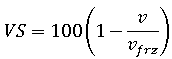
 is specific volume of polymer at the time when either the polymer in element becomes completely frozen or melt pressure in the element becomes atmospheric; is the specific volume of polymer at atmospheric pressure and room temperature. Specific volume at a particular pressure and temperature is calculated using the pvT relationship.
 Crystallization Term
Equilibrium pvT data is not sufficient for describing the volumetric shrinkage of semi-crystalline materials. The amount of volumetric contraction that occurs in these materials also depends on the degree of crystallization. The degree of crystallization in the part is primarily affected by the mold temperature. The shrinkage calculation uses the crystallization kinetics of the material to determine the volume contraction due to crystallinity levels.
Crystallization is a function of both temperature and time. The level of crystallization is determined by cooling rates. Rapid cooling rates are associated with lower levels of crystalline content and vice versa.
In injection molded parts, thick regions tend to cool slowly relative to thinner sections and so have higher crystalline content and hence higher volumetric contraction. On the other hand, thin regions cool very quickly and so have lower crystalline content and hence lower volumetric contraction than that predicted from equilibrium pvT data.
Orientation Term
During shear flow, polymer molecules align themselves in the direction of flow. The extent of this orientation depends on the shear rate to which the material is subjected and the temperature of the melt.
When the material stops flowing, the induced molecular orientation begins to relax at a rate dependent on the material's relaxation time. If the material freezes before relaxation is complete, the molecular orientation is "frozen-in". This frozen-in orientation will result in different levels of shrinkage in the directions parallel and perpendicular to the direction of material orientation.
To determine the level of frozen-in orientation, the Fill+Pack analysis calculates the following quantities for each element and each grid point i across that element at the time when the grid point freezes:
- The shear stress,

- The cooling rate,

- The flow angle,
 , relative to the element's local X-axis. The local X-axis is the direction from the first node number to the second number in the element's definition. Note that the flow direction can be different from laminate to laminate because the growth of frozen layer may change the flow channel and hence the flow direction.
The final level of "frozen in" orientation is determined by taking the molecular orientation level at the time the material stops flowing, which is proportional to the shear stress at that time, and reducing the level of orientation by an amount determined by the relaxation characteristics of the material, which is a function of the cooling rate.
 , at each grid point, the orientation measure,
  , at grid point i and in the direction parallel to the local X-axis is then given by:
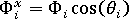
The orientation measure in the perpendicular direction, , is determined in a similar way.
 and
and  respectively, is then determined by summing the grid point measures, that is,
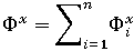
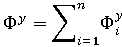
where n is the number of grid points in the plastic.
 , is then defined to be:
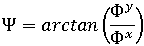
Mold Restraint Term
While the part is in the mold, it is assumed that it cannot physically contract in the plane of the element. However, contraction in the thickness direction is allowed.
As the material contracts, residual stresses build up in the part. The temperature history of a plastic element during the filling, packing and cooling phases affects the rate at which these stresses can relax. A measure of mold restraint is calculated by adding contributions from a number of small temperature increments, in which the rate of relaxation is determined from the current temperature.
Equivalent Thermal Strains
The residual strain shrinkage model described above gives, for each element, a value of parallel and perpendicular shrinkage that represents an average value through the thickness of that element. In reality the level of shrinkage varies through the thickness. If this shrinkage distribution is asymmetric about the cavity centerline, a bending moment is created which may influence the warpage of the part.
Where:
T(z) is the temperature distribution in the plastic when the center freezes, that is, when the element is fully frozen, as obtained from Cool analysis. The peak value of T(z) is the freeze temperature of the material and will be located at a position across the element thickness as determined from the Cool analysis. In evaluating the above equation, the temperature at each mold-cavity interface is approximated to be the end of cycle mold temperature and the temperature distributions either side of the maximum temperature are approximated by parabolic curves.
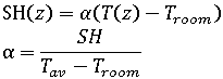
 is the average of T(z) over the thickness,
SH is the average shrinkage as predicted by the shrinkage model,
SH(z) is an "effective" coefficient of thermal expansion. It is not a true thermal expansion coefficient because it includes the effects of other shrinkage processes, e.g. crystallinity.
This SH(z) distribution is then linearized, i.e. converted into a straight line, in such a way as to preserve the bending effect of the distribution. The bending effect is characterized by the integral:
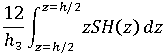
where h is the element thickness.
Note that this conversion to a straight line is not an approximation but a necessity, because the elements types supported by the Autodesk Simulation Moldflow stress analysis program (like most stress analysis programs) can only handle a linear distribution of strain through the thickness of the element.
The result of this linearization is a straight line shrinkage distribution, SHL(z). This is converted back to a linearized temperature distribution TL(z) using the above equations. The reason for converting back to a temperature distribution is historical; ABAQUS only accepts coefficients of thermal expansion and temperature change, not direct initial strain input.
The top and bottom temperature of the element, as determined from TL(z), the room temperature, and the  values for the parallel and perpendicular directions are saved as input for the Warp analysis. In the Warp analysis, SHL(z) is reconstructed from these values using the two equations at the start of this section.