Boundary element method derivation

Cool is a true 3D mold cooling analysis product. It uses a numerical method developed from BEM (Boundary Element Method). From a physical point of view, BEM treats all boundaries as heat sources (gain / loss heat) during the solution.

The temperature in the mold is determined by combining the influence from all sources.

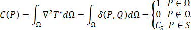
The equilibrium temperature field of a 3D mold can be represented by Laplace's equation: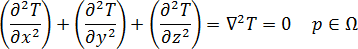

where:

• is the temperature
• is the Laplace operator
• represents the surface area and the inside of the mold

The above equation refers to a specific point in that area, , with boundary conditions unified as:

where:

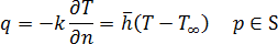
• is the thermal conductivity of the mold material
• denotes the outward normal derivative on the mold boundary,
• is the equivalent heat transfer coefficient on the mold boundary,
• is the equivalent temperature of the ambient environment,
• represents a specific point, and
• is the mold surface (boundary)

To understand how BEM applies all boundary conditions to the solution of the mold temperature field, let us start with the weighted residual expression: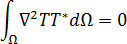

Where is the weighting function.

By making use of Green's second identity, equation 3 can be transformed into the following form: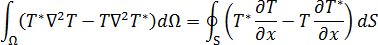

Choosing as the fundamental solution of equation 1 defined by: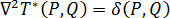

where is a Dirac delta function. For a 3D mold, this can be described as:

where:

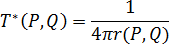
• and are two points in the space, and
• represents the distance between the two points,

Then equation 4 can be simplified as:

where:

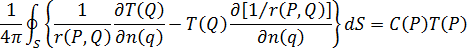
• , and
• is a constant in proportion to the interior solid angle.

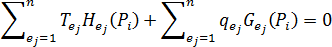
Now equation 7 only has boundary integrations. So if we divide all mold surfaces, , into elements, and assume the temperature and temperature gradient are constant over each boundary element, then equation 7 can be discretised into the following form:

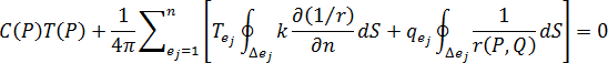
where

• is a specific element
• is the thermal conductivity of the mold material
• is the temperature of element

The temperature influence term (or so-called H term), which represents the influence strength of temperature on element to point , is given by the expression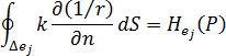

The heat flux influence term (or so-called G term), which represents the influence strength of heat flux input on element to point , is given by the expression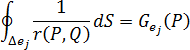

Suppose is the centroid of element . If we substitute in equation 9 with , then we can get linear equations as: