Parameters of time history analysis

Select a time history analysis and click OK in the New case dialog or click Parameters in the Analysis Type dialog to define its parameters for a new dynamic load case of a structure..

The Time History Analysis dialog contains the following parameters.

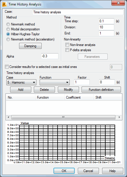
An editable Case field containing the load case name.
The Method field to select a method of carrying out time history analysis. Modal decomposition is the default value. Click Damping to determine detailed damping values of individual vibration modes for the modal decomposition method or Rayleigh factors for the Newmark and the Hilber-Hughes-Taylor (HHT) methods. If the HHT method is applied, it is necessary to define the α coefficient.

If the time history analysis includes a definition of a load in the form of a forced displacement, velocity, or acceleration of supports, then the HHT (Hilber-Hughes-Taylor) or Newmark (acceleration) method should be chosen. Modal decomposition method does not take those loads into consideration.

The Time field contains the following parameters.

Time step - The step of time variable for which the results are stored.

Division - The number of time step divisions defining the storage frequency of analysis results.

End - The end value of time variable for which the analysis is carried out.

If a method other than modal decomposition is selected, then the number of time step divisions (time step of saving results) is specified in the Division field to define the time step of integration. The time step of integration equals Time step / Division. When the division value equals 1, the time step of saving results is identical as the time step of integration.

If modal decomposition (linear time history analysis) is selected, the algorithm calculates the maximum value of the time step of integration for each mode, equaling the value of period divided by 20. This guarantees stability and the precision of results. Calculated step value is divided by the division value. The value received (step_1) is compared to the time step of saving results. A The smaller of these values ( step_1 and time step of saving results) is adopted as the time step of integration. Take note that if the first value is applied in calculations, it is slightly modified so the time step of saving results is a multiple of this value.

List of the available simple static load cases or masses in directions X, Y or Z.
List of the defined time functions and a preview of the diagram of the selected function.
Coefficient field.
Phase shift field.
Function definition.
A table containing the following columns.

Case - Indicates the number of the selected load case or mass direction

Function - The name of the time function selected for the given load case

Coefficient - The incremental coefficient for time function value for the given load case; the default value of the coefficient = 1.0

Phase - Phase shift of the time function for the given load case; the default value = 0.0.

In addition to the listed parameters, there are non-linear analysis options available (see non-linear time history analysis).

Non-linear analysis - Considers influence of the axial force.

P-Delta analysis - Considers influence of square elements of the equation.

Click Parameters in the Non-linearity field to open the Options of non-linear analysis algorithms dialog (see also: Non-linear analysis algorithms), to define parameters of the methods applied to solve the equation system.

For example, to carry out the time analysis of the responses of a structure to an explosion, you can define a load case corresponding to air pressure on the structure and the explosion variability function. Analysis of structure behavior during an earthquake is another example. In this case, you can define time functions for selected mass directions generated on the base of seismograms.

Select a static load case or mass direction and click Add to define the function. You can also modify and delete active table rows by clicking the appropriate buttons.