The material property input dialog box for the hyperelastic and foam material models include a Curve fit routine. The curve fit is used to determine the constants for the mathematical material model by performing a best-fit calculation of the user-supplied stress-strain data for the material. Keep in mind that no solution will fit the test data exactly! Variations in the tests and materials will produce scatter in the test data. Therefore, a high degree of precision in the curve-fitting routine is not justified in most situations. What is important is that the results of the curve-fitting routine follow the test data in the range of interest.
Each material model has options specific to its needs; some of the items described below will not be relevant depending on the material model. The general layout of the Curve Fit dialog box is shown in Figure 1 and described below.
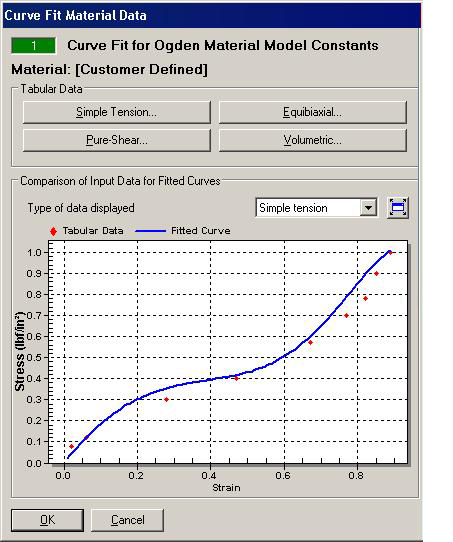
Figure 1L: Curve Fit dialog box for Ogden (left half of dialog box)
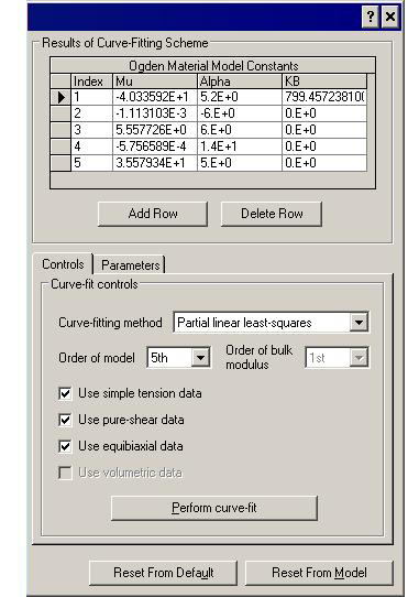
Figure 1R: Curve Fit dialog box for Ogden (right half of dialog box)
Tabular Data Section:
This section is used to enter the known stress-strain data for the material. First, it is important to keep the following statements in mind when obtaining the test data:
- To derive accurate constants for the analysis, stress-strain data entered into the Curve Fit must cover the complete range of loading that will be encountered in the analysis. For example, if the part will experience shear stresses in addition to tension and compression, then Pure-Shear stress-strain data must be entered. Simple Tension by itself is not sufficient to properly model the behavior of the material in such situations. The same is true for the other types of tabular data.
- Since the data from all the experiments are used together to derive the material constants, it is important that the material tested be from the same batch. Otherwise, variations in the material production will skew the test data.
- Many elastomers change behavior during the first several loading cycles. Also, the stress-strain curve changes when the maximum strain experienced is increased. Thus, the material should be cycled to a strain value expected in the analysis, and the load should be repeated until the behavior stabilizes.
- If not already provided as such, the stress-strain test data may need to be shifted to a zero strain condition. When a hyperelastic material is stretched to a new strain rate, it often will not return to the original strain. (This is true whether it is the first cycle or after many cycles; it is the new higher strain rate that causes a new permanent deformation.) The permanent deformation that is measured in the test needs to be removed from the strain values. Likewise, the changing cross-sectional area due to the permanent deformation needs to be reflected in the initial area used to calculate the stress. These two corrections will shift the stress-strain curve back to a starting value of 0,0.
- Depending on the material model used, most of the hyperelastic material models do not change properties due to repetitive loading. Each cycle in the analysis follows the calculated stress-strain curve. Thus, the test data may need to be chosen or averaged to match the analytical behavior.
- Most hyperelastic material models follow the same stress-strain curve for loading and unloading. There is no permanent deformation.
The types of test data that can be entered are as follows:
- Simple Tension button: Enters the stress-strain data from a simple tension test. The test data must be such that a pure state of tensile strain is measured. No lateral constraint exists in the test data. Only the tension branch is entered. Compression data is derived from the equibiaxial data.
- Equibiaxial button: Enters the stress-strain data from an equibiaxial or equal biaxial extension test. This is the test data that is used to reproduce the compression stress-strain. By pulling equally in two directions, a state of strain equivalent to pure compression is created.
- Pure-Shear button: Enters the stress-strain data from a pure shear strain test. For hyperelastic materials, this is typically a wide tensile specimen, but because the material is nearly incompressible, a state of pure shear exists.
- Simple Shear button: Enter the stress-strain data from a simple shear test.
- Volumetric button: Enters the pressure-strain data from a volumetric compression test. This data is used to determine the bulk modulus. For hyperelastic materials, it is important for situations in which the material is slightly compressible or situations in which the part is highly constrained. The bulk modulus is typically two to three orders of magnitude greater than the shear modulus. For foam materials, the volumetric data is important to capture the compressibility of the foam.
Clicking any of the buttons in the Tabular Data section will bring up a new dialog box in which the stress and strain data is entered. The controls available are as follows:
- Strain format pull-down: Select the format for the strain data. Nominal strain is calculated from (change in length)/(original length), and Stretch is calculated from (current length)/(original length) = 1+(Nominal strain).
- Effective Poisson's Ratio field (foam material models only): If the Poisson's Ratio is known and the transverse strain is unknown, then enter an effective Poisson's Ratio value. This input is used in conjunction with the Populate button and primary strain entered in the spreadsheet to calculate the transverse strain.
- Populate button: Clicking this button will calculate the values for the Strain, Transverse column in the spreadsheet based on the Effective Poisson's Ratio field and the Strain, Primary spreadsheet column.
- Input Transverse Stress check box: For foam materials, the shear stress and transverse stress can have different values. When this option is activated (it only appears on the Simple Shear test data), the transverse shear stress is entered in the stress-strain spreadsheet. When the option is not activated, the transverse shear stress is assumed to be identical to the shear stress, and the column is not included in the spreadsheet.
- Stress-Strain Data or Volumetric Pressure-Strain Data spreadsheet: Enter the stress and strain requested (depends on the type of data). Engineering stress and strain should be used (based on the original length and area.) The values should be entered in ascending order based on the second column (generally strain for hyperelastic materials and stress for foam materials).
- Auto-correct check box: for volumetric pressure-strain data, the sign of the strain and pressure need to be correct to calculate the correct bulk modulus. When this option is activated, the processor will switch the sign of the input volumetric pressure if needed to get the correct calculation. If not activated, the strain values should be negative and the pressure should be positive.
- Add Row and Delete Row buttons: Adds a row to the end of the spreadsheet and deletes the current row, respectively.
- Sort button: Sorts the stress-strain data in ascending order based on the second column (generally the strain value for hyperelastic materials or the stress value for foam materials).
- Import button: Imports the stress-strain data from a comma-separated file (CSV). The data file should be in the same format as the spreadsheet, but without the Index column. Note that any existing data is replaced with the imported data. For the foam material models, two or three columns can be imported. If the third column - Strain, Transverse - is not in the comma-separated value file, the column will be set to zero. Use the Effective Poisson's Ratio field and the Populate button to create estimated values. Attention: Some of the stress-strain spreadsheets use stress in the first column and some use strain. The .CSV file needs to have the data in the proper column to correspond to the spreadsheet.Tip: The values in the comma-separated file are imported using the active Display Units. Change the Display Units if necessary before importing the data. For example, a value of 314 is imported as 314 psi if the Display Units are set to pound and inch, and 314 Pa if the Display Units are Newton and meter.
- Export button: Saves the entered stress-strain data to a comma-separated file.
Parameters Tab
Some of the material models need estimated or guessed values to start the least-square fitting routine. These parameters are entered on the Parameters tab and should be provided before attempting the curve fit. Which parameters are entered depends on the Curve-fitting method algorithm chosen on the Controls tab.
Partial linear least-squares: This search method computes all possible combinations of coefficients based on the initial guesses, and reports the combination that gives the minimum error. Since all combinations are computed, this method may take longer than the other methods, especially if a large increment value is used. Also, note that solutions outside of the range are not tested, so a solution with a smaller error may exist. If the plotted results do not fit the data, try a different range. The input is as follows:
- Estimate or Guessed values: Enter the initial estimate or guess for the parameter. This input is actually the middle of the range that is computed. Note that a value of 0 may not be acceptable for some values in some material models. For example, the potential equation for the Ogden material model uses the parameter alpha in the denominator, so dividing by zero would not be acceptable. If such cases arise during the fitting routine, the parameter will be switched to the pre-defined default values.
- Range value: Enter the range of guess values that are tested (the lowest value tested to the highest value tested). The lowest value is equal to the guess value minus half the range, and the highest value is equal to the guess value plus half the range.
- Increment value: This is the number of points between the lowest value and the highest value that are calculated. So an increment of 20 for three parameters would create 20^3 = 8000 combinations from which the minimum error is reported.
Levenberg-Marquardt algorithm, Gauss-Newton algorithm, and Constrained Optimization: These methods start at the initial guess and locate the first minimum (slope of the error function is zero) to the best fit equations. Since there may be numerous minima when multiple variables are involved, the accuracy of the solution is dependent on the initial guesses. See Figure 2.
- Estimate or Guessedvalues: Enter the requested estimated or guessed value for each of the constants. It is best to not use a value of zero. In addition a non-zero value should be entered for each guess according to the order of the model. If calculating a 5th order model, then estimates should be entered for the first 5 constants. A good estimate is the results from another curve fitting method. For example, the constants found using the Partial linear least-squares method are a good estimate for the Levenberg-Marquardt algorithm. Since the curve fit is a numerical solution technique, a different estimate can result in a different curve fit result.
- Maximum Iteration field: Enter the maximum number of iterations to use. If a solution is not found before reaching the maximum number of iterations, then an error will be given during the curve fitting routine.
- Tolerance field: Enter the tolerance to use for the curve fitting routine. The solution is considered to be converged when each of the constants changes by a value less than the tolerance from one iteration to the next.
Error
 Value
Value
Controls Tab
Curve-fit controls Section:
The curve-fit controls are used to indicate how the test data is to be used for the curve fitting routine, such as which test data to include in the curve fit calculation, the order of the model, and the method for fitting the data.
- Use data check boxes: Activate the check boxes for the test data to use in the curve fitting routine. All test data entered should be used. The only reason to not use a particular set of data is if one set causes a poor fit to the other data. In this case, a different order of model, different curve-fitting method, or material model should be used to get a better fit.
- Curve-fitting method drop-down: Choose a numerical technique to find the best fit to the test data. Each technique will give a different set of constants; the method that gives a good fit to the data (visually and in the RMS) is the one to use. Note that the Levenberg-Marquardt algorithm and the Gauss-Newton algorithm can be sensitive to the initial estimate; enter these on the Parameters tab. The Partial linear least-squares method can be good for finding the initial estimates for the constants.
- Order of model pull-down: Select the order of the model for the curve fitting routine. In general, the lower the order, the faster the analysis, but higher order models are required to get a better fit to the test data, especially when the stress-strain curve has more inflection.
- Order of bulk modulus pull-down: Select the order of the bulk modulus calculation for the curve fitting routine. Higher order will give a more accurate fit to the test data. Some material models cannot estimate this value unless the volumetric test data is provided; other material models will default this entry to 1-constant unless the volumetric test data is entered and used in the curve-fit.
- Perform curve fit button: Click this button to begin the curve-fit operation. The Curve-Fitting Process dialog box will appear. Then, click the Fit button to start the iterative process. If it succeeds, the accuracy of the curve fit will be given (root-mean-square); smaller values indicate a more accurate fit to the chosen data. If it does not succeed, then change the initial guesses on the Parameters tab and try to perform the curve fit again. Note: Curve fitting uses various least-square fitting algorithms to determine the material constants. As such, various numerical techniques and input parameters may result in different solutions. Some tweaking of the values may result in a different curve fit. Since the test data includes variations due to uncontrollable factors, differences in the curve fitting routine are usually negligible. (Refer to numerical method textbooks or Web sites for details on the curve fitting methods.)
Results of Curve-Fitting Scheme Section
The material model constants calculated by the curve fitting are shown in this section. To see the effect that the constants have on the fit to the data, change a value and choose a Type of data displayed to update the graph.
These values will be copied from the Curve Fit Material Data window to the Element Material Specification window when the OK button is clicked to close the Curve Fit Material Data window.
The following equations are used for the various material models:
- Neo-Hookean
- Uniaxial: Tu = stress = 2(λu - λu2)C10, where I1 = λu2 + 2λu-1
- Equibiaxial: TB = stress = 2(λB - λB-5)C10, where I1 = 2λB2 + λB-4
- Pure Shear: TS = stress = 2(λS - λS-3)C10, where I1 = λS2 + 1 + λS-2
- Volumetric: p = pressure = -K(J-1), where J = λv3
where λ = stretch = 1 + strain
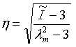
- Van der Waals:
- Uniaxial: where I1 = λu2 + 2λu-1 and I2 = λu-2 + 2λu
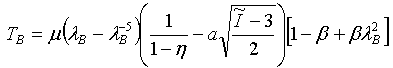
- Equibiaxial: where I1 = 2λB2 + λB-4 and I2 = 2λB-2 + λB4
- Pure Shear: where I1 = λS2 + 1 + λS-2 and I2 = λS2 + 1 + λS-2
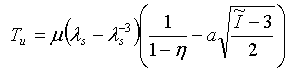
- Volumetric: p = pressure = -0.5K(J-1/J), where J = λv3, where
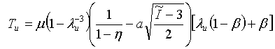
- Uniaxial:
![]()
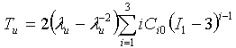
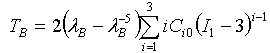
- Yeoh:
- Uniaxial: where I1 = λu2 + 2λu-1
- Equibiaxial: where I1 = 2λB2 + λB-4
- Pure Shear: where I1 = λS2 + 1 + λS-2
- Volumetric: where J = λv3
- Uniaxial:
Comparison of Input Data for Fitted Curves Section
This section displays the tabular test data and the fitted curve. Use the Type of data displayed drop-down to choose what to display in the graph. Any type that has data entered can be displayed regardless of whether that data is used in the curve-fit or not. (Naturally, data that is not used in the curve-fit routine is unlikely to have constants that fits the data very well. The fitted curve will likely not follow the tabular data very well.)
The graph is not updated automatically if the material model constants are changed manually. To update the graph, re-select the Type of data displayed.
Curve Fit Example
Let's go through an example using simple tension, equibiaxial, and pure shear test data with an Ogden material model.
- Set a model with brick or 2D elements to the analysis type of nonlinear (either Static Stress with Nonlinear Materials or MES with Nonlinear Material Models.) The test data is given in MPa, so the model units should be Newtons and millimeters. (1 MPa = 1 N/mm^2)
- Edit the element definition. Right-click Element Definition for the part and choose Edit Element Definition. Set the Material model to Hyperelastic: Ogden. Click OK.
- Edit the material properties. Right-click Material for the part and choose Edit Material. Choose [Customer Defined] and click Edit Properties button. If the Ogden material model constants were known, they could be entered directly. Since we have the material test data (given below), click the Curve fit button.
- To enter the simple tension stress-strain test data, click the Simple Tension button. Either add rows to the spreadsheet and type the data given below, or copy and paste the text below to a text file (with .CSV extension) and use Import to read in the data. Click OK when done.
- Enter the equal biaxial stress-strain test data in a similar fashion. Click the Equibiaxial button. Either add rows to the spreadsheet and type the data given below, or copy and paste the text below to a text file (with .CSV extension) and use Import to read in the data. Click OK when done.
- Enter the pure shear stress-strain test data in a similar fashion. Click the Pure-Shear button. Either add rows to the spreadsheet and type the data given below, or copy and paste the text below to a text file (with .CSV extension) and use Import to read in the data. Click OK when done.
- On the Controls tab, activate the check box for each of the test data.
- For the Ogden material model, the Curve-fitting method of Partial linear least-squares is a good starting point because it requires an estimate for just one of the parameters (the Alpha value). So choose that method from the pull-down. Leave the other settings at the defaults. Note that the Order of bulk modulus is grayed out because volumetric data was not entered.
- On the Parameters tab, set the Guessed Alpha, the Range value, and the Increment as follows. This will give a moderately wide range of values for the solution to use, and an increment of 20 will be a rough but good approximation for the first run without taking too long to calculate all the permutations. Note that the guess values are the defaults for the Ogden material model.
Order Guessed Alpha Range value Increment 1 1.2 10 20 2 -2 10 20 3 6 10 20 - On the Controls tab, click the Perform curve-fit button, and then the Fit button. The Root-mean-square error is 0.184: relatively large compared to the maximum stress. Click the Done button.
- Using the Type of data displayed pull-down, review the graph for each of the curve fit data (simple tension, equibiaxial, and pure shear). The curves follow the test data reasonably well (the Equibiaxial is off the most), so the constants found are the right order of magnitude.
- With a good estimate in hand, switch the Curve-fitting method to Levenberg-Marquardt algorithm. Then enter the guess values on the Parameters tab using the solution found previously. Since precision is not required for the estimates, the following rounded-off values will suffice:
Order Guessed Mu Guessed Alpha 1 -0.16 6.2 2 4.4 0.5 3 0.026 9 - On the Controls tab, click the Perform curve-fit button, and then the Fit button. The Root-mean-square error is 0.183: hardly any better than the previous fit. But, notice how this solution method is much faster than the Partial linear least-squares method.
- Additional trials could be performed using different initial values to find alternate minima, but it seems more productive to try a higher order model. On the Controls tab, set the Order of model to 5th and the curve-fitting method to Partial linear least-squares. Then on the Parameters tab, enter guess values as follows. Two notes. First, because the order of the model was changed, the constants found with the previous solution are generally not relevant guesses in a more efficient solution algorithm like the Levenberg-Marquardt. It is better in this case to start over with the Partial linear least-squares. Secondly, note that the increment value was lowered from before. Since the calculation is doing every combination of the first order alpha with every combination of the second order alpha and so on, a fifth order solution can quickly create a lot of calculations! The smaller increment value is used to minimize the time the curve-fitting routine takes.
Order Guessed Alpha Range value Increment 1 1.2 10 10 2 -2 10 10 3 6 10 10 4 19 10 10 5 1 10 10 - On the Controls tab, click the Perform curve-fit button, and then the Fit button. The Root-mean-square error is 0.142. As expected, each of the curves under the Type of data displayed fits the test data better. The results are shown in Figure 1. Additional trials could be performed, but considering the accuracy of the test data, this curve fit should be acceptable.
Simple Tension Test Data
0,0
0.02,0.08
0.06,0.12
0.28,0.30
0.47,0.4
0.67,0.57
0.77,0.7
0.82,0.78
0.85, 0.9
0.89, 1.0
Equibiaxial Test Data
0,0
0.02,0.14
0.06,0.25
0.12,0.4
0.28,0.6
0.43,0.8
0.57,0.95
0.65,1.16
0.72,1.4
0.80,1.72
0.89,2.4
Pure-Shear Test Data
0,0
0.02,0.08
0.07,0.2
0.20,0.37
0.59,0.71
0.73,0.92
0.83,1.1
0.89,1.28