The reinforced concrete material model is treated as statistically homogeneous with different tensile and compressive behaviors. It follows a smeared crack model where cracking and crushing are simulated via degeneration of the elasticity at integration points instead of tracking individual macroscopic cracks. The model described here is intended for relatively monotonic loadings. (A true monotonic load either increases or decreases but does not reverse.) In the current model, cracking is considered the most important aspect, but compression under confinement is also reasonably accounted for.
The reinforced concrete material model also implements a smeared rebar approach. The rebar is assumed to be distributed (smeared) over entire element with a given volume fraction. The strength of the rebar reinforces the concrete in the specified direction. The rebar material itself follows an elastoplastic material model with von Mises isotropic hardening. Three independent directions of rebars can be defined.
Figure 1 shows a typical uniaxial behavior of plain concrete. When concrete is loaded in compression (points 3-2-1), it behaves elastically until it reaches the yield point (point 2). The material response softens and nonrecoverable deformation occurs. After reaching the failure point at the peak strength (point 1), the material deteriorates but can still theoretically carry some loads. This compression softening is not currently modeled by the analysis, and the concrete is considered to be crushed and no longer able to carry any loads after this point. Unloading before failure is assumed to be elastic and follows the Young's modulus.
When concrete is loaded in tension, it behaves elastically until it reaches the failure strength (point 4). Post-failure behavior in tension (tension softening) is very important in modeling load transfer across cracks (tension stiffening) in reinforced concrete.
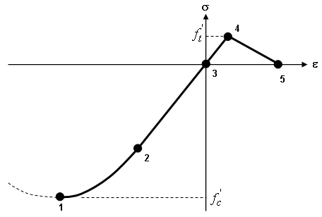
Figure 1: Idealized Uniaxial Behavior of Plain Concrete
Failure Criterion
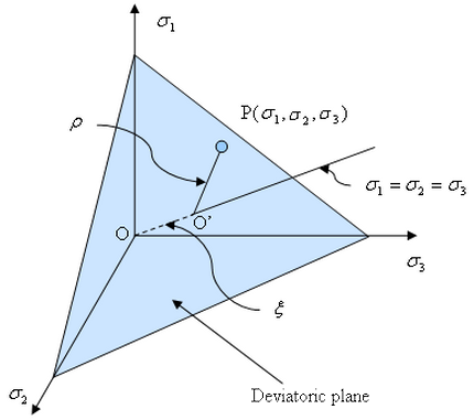
It is convenient to work in the principal stress space, where any stress state is defined by Haigh-Westergaard coordinate (x, r, q):
 (1)
(1)
where I1 = δijσij, J2 = 0.5SijSij, J3 = (SijSjkSki) / 3, and Sij = σij - (δijσkk) / 3.
|
(a) Principal stress space |
|
(b) Deviatoric plane with principal stress projected on |
| Figure 2: Haigh-Westergaard Stress Coordinates |

The analysis uses a similar failure criterion to that of Hsieh-Ting-Chen (HTC) four-parameter criterion (reference 1) but the effect of -dependency is introduced via the deviatoric radius representation of Willam and Warnke (reference 2).
 (2)
(2)
 (3)
(3)
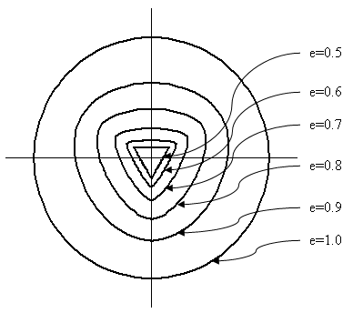
where ft' and fc' are the uniaxial tensile and compressive strength (absolute values), respectively; and e is the eccentricity as defined by Kang and Willam:
 (4)
(4)
where c 0 is a material constant that can be calibrate from experiments (it is set to 5.5 in Kang and Willam, reference 5). The equi-triaxial tensile strength ζ 0 =sqrt(3)f t '. The eccentricity of 1 is a circle in the deviatoric plane (Figure 3) and failure is then independent of the Lode angle ϑ.
The loading of yield surface is assumed to be an expansion from the initial yield surface to the final failure surface via a single parameter k, whose value ranges from k 0 at the initial yield to 1 at failure. Following Imran and Pantazopoulou (reference 4), the intersection of intermediate failure surfaces with the hydrostatic axis is controlled by an additional term.
 (5)
(5)
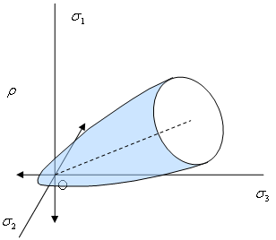
In addition, the analysis also assumes no yielding for tension-dominant status via introducing a tension cut-off (maximum tensile stress, or the Rankine criterion). In the mixed tension-compression region (reference 1), the yielding surfaces gradually evolve. The failure envelop is thus an open surface in the principal stress space as demonstrated in Figure 3. The analysis always assumes the failure is cracking when principal tensile stress exists. This is a little arbitrary since concrete fails in complicated ways and as a result some studies do not distinguish the failure types.
|
(a) Concrete failure envelope |
|
(b) Deviatoric view of concrete failure envelope |
| Figure 3: Failure Envelope |
Compression Hardening
For simplicity, associated flow and isotropic strain hardening are used when concrete is under dominantly compressive loading. This approach yields symmetric governing equations and is computationally efficient. However, it generally over-predicts the plastic volume strain.
In the mixed tension and compression domain (reference 1), the yield surface is modified to be the tangential surface to the original at the boundary (Figure 4).
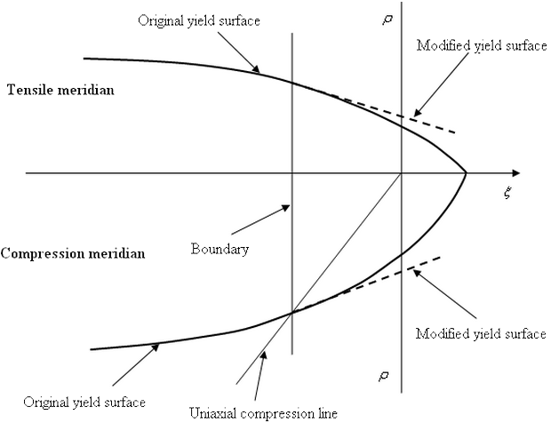
Figure 4: Yield Surface in Mixed Tension-Compression Domain
The stress update is through the fully implicit backward Euler return mapping scheme, which requires quite significant amount of computation.
Tension Stiffening
Cracking is assumed to occur when at least one principal stress is tensile at the failure surface. The analysis uses damaged elasticity to model the cracked concrete. It is assumed that no permanent strain is related to cracks.
To overcome the mesh-sensitivity related to the tension softening, the analysis assumes that the fracture energy (per unit area), Gf, is a material property. The specific fracture energy (per unit volume), gf, is related to Gf via:
 (6)
(6)
where l* is the characteristic length or crack band width at integration points (reference 6).
The shear retention coefficient b is specified by the user. A value of 1 stands for perfectly rough crack where shear force can be transferred without loss. A value of 0 represents a perfectly smooth crack where no shear force can be transferred. The Poisson’s effect (lateral expansion) with related to the cracking is neglected. When the crack closes, the compressive stress can be completely transferred.
Stress components associated with an open crack are not included in the definition of the failure surface for detecting further cracking at the same integration point.
Calculating Failure Envelopes
As indicated above (equation 2, with ρ = 0), a3 is determined from equi-triaxial state. Other failure surface parameters (a1, a2, and c0) are solved from nonlinear equations (equation 2, 3, and 4) at three independent stress states. For other combinations of experiments, the user will have to calculate and then input the parameters directly.
For the hardening parameters (a4 and k0), the analysis assumes a non-uniform work hardening as governed by the additional hardening term (equation 5). For simplicity, it is assumed that the dependence of hardening on the effective plastic strain (![]() ) and hydrostatic pressure (ζ) are separable. The effective plastic strain (
) and hydrostatic pressure (ζ) are separable. The effective plastic strain (![]() ) only affects the hardening parameter k. Therefore, users can calibrate a4 and k(
) only affects the hardening parameter k. Therefore, users can calibrate a4 and k(![]() ) based on the uniaxial compression experiment.
) based on the uniaxial compression experiment.
References
- Chen, W.F. and Han, D.J., Plasticity for structural engineers, Springer, 1998
- Willam, K. and Warnke, E., Constitutive model for triaxial behavior of concrete. International Association for Bridge and Structural Engineering, Zurich, pp.1-30, 1975
- Kupfer, H. and Gerstle, K., Behavior of concrete under biaxial stresses, Journal of Engineering Mechanics, v99, n4, pp 853-866, 1973
- Imran I. and Pantazopoulou S., Plasticity model for concrete under triaxial compression. Journal of Engineering Mechanics, v127, n3, pp. 281-290, 2001
- Kang, H. and Willam, K., Localization characteristics of triaxial concrete model, Journal of Engineering Mechanics, v125, n8, pp941-950, 1999
- Crisfield, M.A., Non-linear finite element analysis of solids and structures, Vol. 2: Advanced topics, J. Wiley & Sons, New York, 1997