Event simulation is engineering by simulating a physical event in a virtual laboratory. To perform an engineering analysis using event simulation requires a different viewpoint from classical stress analysis.
In engineering education, we are taught that stress is a function of force, or ![]() σ= f(force). Deformation, or displacement, is another function of force, or d = g(force). In event simulation, however, we assume that the design force is indeterminate and results from some type of action or motion. In this scenario, force and stress are functions of displacement or deformation; that is force = f(d) and σ = g(d). The deformation or displacement is calculated directly from the governing physics equations.
σ= f(force). Deformation, or displacement, is another function of force, or d = g(force). In event simulation, however, we assume that the design force is indeterminate and results from some type of action or motion. In this scenario, force and stress are functions of displacement or deformation; that is force = f(d) and σ = g(d). The deformation or displacement is calculated directly from the governing physics equations.
Contrast Mechanical Event Simulations with Classical Methods
Let's use a simple cantilever beam to highlight the differences between classical stress analysis and event simulation.
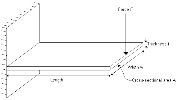
An engineering handbook shows for a cantilever beam subjected to a force at the end opposite the fixed end the maximum stress (at A) is given by:

|
[1] |
where M is the moment generated by the force F (M = Fl), c is the distance from the neutral axis to the edge of the beam (c = t/2), and I is the area moment of inertia (I = wt 3 /12). This result is obtained by considering the bending of a beam with Hooke's law (|F| = k|d|). This law states that force is a linear function of displacement. This statement forms the basis of classical stress analysis and modern finite element stress analysis.
In finite element analysis, the matrix equation {F} = [K]{d} is solved for the displacement vector, {d}, from the force vector, {F}, and the stiffness matrix, [K]. After, the stresses are calculated from the equation {σ} = E{ε}, where {ε} is the strain vector, which is a normalized displacement vector. E is the modulus of elasticity, which corresponds to the Hooke's law constant, k.
All is well if the beam is always at rest, which is the only valid application of equation [1]. In practical mechanical engineering, the static case never dictates the design. The design must consider the worst case scenario, which generally occurs when the beam is in motion, and the forces, and thus the stresses, are greater than those under static conditions.
Here is where event simulation enters the design process. You can simulate the entire event, not simply obtain a static solution. A useful by-product of simulating the event is the forces generated by motion. According to Newton's second law,
F = ma [2]
or force equals mass multiplied by acceleration. Mass is an inherent property of matter, and acceleration is the rate of change of velocity. This law quantifies the fact that mass is the property of matter that causes resistance to changes in motion. Note that under the influence of gravity, a body at rest of mass m generates a force mg, where g is the acceleration due to gravity. In the special cases of constant acceleration (gravity field near the surface of the book) and short-lived events (say of length Δt), Equation [2] can be rewritten as
[3]
where Δv is the amount by which the velocity changes during Δt time. A force of 1,000,000 lb. acting over 0.000001 seconds produces the same impulse (or change in momentum) as a force of 1 lb. over 1 second.
Event simulation relies on the combination of Newton's second law with Hooke's law as follows:
F = ma = -kd, or
ma + kd = 0
[4]
The negative sign in front of k is because the force is in the opposite direction of the displacement. Also, note that the nebulous quantity force can be eliminated, and that the concept of time has been introduced through the acceleration. To simulate real world problems, you must also take damping or friction into account. Such dissipating forces can be modeled by:
F = -cv [5]
where v is the velocity and c is a constant; note how dissipation also opposes motion. Combining equations [4] and [5], we obtain:
ma + cv + kd = 0 [6]
or in matrix form:
[M]{a} + [C]{v} + [K]{d} = 0 [7]
It is the basic equation of virtual engineering. Note how it models the combination of motion, damping, and mechanical deformation. If the stresses are still of interest, calculate them at any time during the analysis by application of the formula {σ} = E{ε}, where {ε} (the strain vector) is easily obtained from the displacement vector {d}. Virtual engineering provides a means to design for the worst case scenario. Even for the simple example of the cantilever beam, the solution of equation [7] is beyond the realm of hand calculations. But, with current computer technology, the solution of more complex problems is reduced to the practical level.
Numerical Example
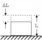
We consider a numerical example to demonstrate the power of virtual engineering. Imagine a cube of mass m impacting a rigid surface along a face. We are interested in the maximum deformation experienced by the cube. We first perform a hand calculation for the maximum compression length. Then we use virtual engineering to solve the same problem and compare results.
|
Cube before contact. |
Cube at time of maximum deformation. |
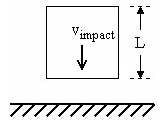
By Newton's second law, the impact force is given by equation [1]. Following the principles of classical physics, we assume that the entire mass of the cube is located at its centroid. If we also assume that for any particular location on the cube the acceleration is constant throughout the impact, then equation [1] takes the form:

[8]
where Δv is the change in velocity of the top of the cube during the impact interval, Δt The factor of 1/2 in equation [8] is needed because we are applying equation [1] at the centroid, half-way up the cube we expect half the acceleration to that at the top face. In other words, once contact is made, we expect the top of the cube to move twice as fast as its centroid. The constant acceleration assumption combined with basic kinematics allows us to obtain an expression for the amount by which the cube deforms during impact:
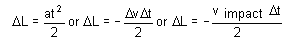
[9]
where v impact is the velocity of the cube, and thus of its top face, at the moment that contact is made. The negative sign in equation [9] is needed because Δv is negative and we seek a positive value for ΔL. Note how Δv has been replaced by just v impact because at the time of greatest deformation, the top of the cube is not moving.
By Hooke's law, the force on the cube is given by
[F = -kDL] [10]
Combining equations [8] through [10], yields:
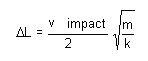
[11]
Putting k in terms of E (k = EL for a cube of length L deforming along an axis perpendicular to a face), one obtains:
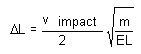
[12]
Using the software, we simulate the same impact problem. We model a cube of length (L) 1.0 in, and mass (m) 0.000253 lbm. It is comprised of a material with a modulus of elasticity,E, of 107lb/in2. The event simulated is actually the dropping of the cube from a height of 100 in. It results in an impact velocity (vimpact) of 278 in/sec. when under the influence of a gravity field of strength 386.4 in/sec2. The software predicts a maximum deformation (ΔL) of 0.000694 in. which compares favorably with the value of 0.000699 in. given by equation [6].
This example demonstrates how difficult it is to analyze a simple impact problem without using digital prototyping software. Imagine how involved, or even impossible, the hand-calculation is for a more complex geometry. You can resort to conventional, classical finite element analysis (FEA). Such an analysis neglects (gross) motion, but might be adequate if we knew the impact force. The inadequacies occur primarily because such an analysis neglects the vibrations set off by fluctuations in the force during the actual impact.
Force Estimation Methods
There are three commonly used methods to estimate force values for input into classical FEA: experience, rigid body dynamic analysis and physical experimentation.
-
Experience
Some engineers rely on prior experience with similar problems to estimate these forces. Usually they rely on safety-factors, hoping that they are sufficient to prevent failure, yet not overly conservative to produce an over-designed part.
-
Rigid Body Dynamics
Rigid body dynamics programs calculate motion-generated forces using a model of the part. To arrive at numerical values for these forces, such programs use vaguely defined stiffnesses. Because these programs are limited by the rigid-body assumption, using these stiffnesses to calculate forces cannot be reliable.
-
Experimentation
Performing an experiment on a prototype of the part is an accurate means by which to obtain these forces. But, such an approach completely defeats the economic savings of using computer analysis.
Conclusions
Event simulation allows one to model an entire physical event with the least number of assumptions. Specifically, one does not have to assume a static situation or have to estimate values for forces that result from motion. Furthermore, event simulation has the useful by-product of generating a frame-by-frame record of the event, not just a snap-shot at its conclusion.