Remote Loads and Constraints

Note: The information in this section applies to all linear and nonlinear analysis types that support remote loads and constraints.

What Do Remote Loads and Constraints Do?

Adds a nodal load or boundary condition to a point in space; a point not on the model.
The point in space is connected to selected nodes on the model with line elements.
You define the properties of the line elements as beam, truss, or similar line elements.
The remote load or boundary condition is transmitted through the line elements to the model.
Remote Loads and Constraints differ from Remote Forces, in which the effects of a remote force are applied directly to the model surface using automatically-calculated nodal forces (no line elements are created).

Since the Remote Load command generates new geometry and a node at the point in space, you can add any number of additional objects at the new point.

Apply Remote Loads or Constraints

Use any of the selection commands (Selection Select) to select where the remote load or constraint is to be distributed onto the model. For example, to apply a torque to the end of a shaft, select the vertices or surface on the end of the shaft. Regardless of what is selected (part, surface, edge, line), the vertices on the selection are used. Most applications require the remote load or constraint to be distributed to three or more vertices not in a straight line.
Right-click and choose the Create Remote Load & Constraint command. This command is also available via the ribbon (Setup Loads Remote Load & Constraint).
Use either of the following methods to specify the location of the remote load or constraint.
- Type the X, Y, and Z coordinates of the desired Load Location. Or,
- Select one vertex or construction vertex in the display area and click the Use Selected Point button. The coordinates of the selected vertex will be listed in the X, Y, and Z fields.
The part, surface, edge, or vertices over which the remote load or constraint is to be distributed are already listed by virtue of starting the command with them selected. However, to change the destination or create a new remote load or constraint, do one or both of the following:
- Select the new location or locations, and click the Add button.
- Select one or more lines in the Load Destination list and click the Remove button.
Specify the Part, Surface, and Layer attributes for the line elements that will connect the remote load to the model. Generally, the default part number is a new (previously unused) number or the same number as previously generated remote load elements.
Click the Generate Elements button. The lines from the remote load location to the model are created.
Click the Add Load button to see the list of nodal loads or boundary conditions that can be added. Some of the available options may not be suitable depending on the analysis type and the type of elements used for the load elements.
If another remote load location is required, repeat the above steps starting with step 3.
Click the Close button when finished applying all remote loads to all remote locations.

Tip: While the Create Remote Load dialog box is opened, multiple loads or boundary conditions can be added to the same node by using the Add Load button more than once. After closing the dialog box, additional loads and boundary conditions can be added to the same node by selecting the vertex at the remote load location (Selection Select Vertices), right-clicking, and choosing the appropriate entry under the Add fly-out menu.

Define Remote Load/Constraint Line Elements

After the remote load or constraint line elements are created, use the browser (tree view) to define the Element Type, Element Definition, and Material. Any line element type can be chosen (beam, truss, gap, and so on), provided it suits the requirements of the analysis. Here are a few guidelines to keep in mind:

Moments can be applied as a remote load, but they can only be transmitted through beam elements. Truss elements, gap elements, and other line element types that do not have rotational degrees of freedom cannot transmit moments and torques. the joints of these element types are pinned (no translation, rotation allowed). (See Getting Started: Introduction to Autodesk Simulation FEA: Nodes and Elements for additional information on transmitting loads, restraints, and degrees of freedom.)
Imagine the array of load elements as being supported by boundary conditions instead of connected to the model. The support reactions at these hypothetical boundary conditions are the loads that are transmitted to the model. The total of these support reactions equals the applied loads, but the distribution of the forces and moments may be affected by the stiffness of the load elements.
Stiff beam elements acts like a rigid structure attached to the model, so the surface (or nodes) of the model where the remote load is distributed tend to keep the same shape but move as a rigid surface. Weak beam elements and truss elements transmits the load but do not completely prevent deformation of the shape of the surface.

Example – Use of Remote Loads and Remote Constraints

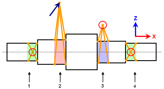
Figures 1 and 2 illustrates how to use remote loads to analyze a shaft (made from brick elements) that is part of a gear train. In the FEA Model, the two boundary conditions at the bearings prevent the shaft from rigid body translations in all directions. The bearing on the left is held radially (Ty and Tz) and axially (Tx, to contain thrust loads), and the mounting of the bearing on the right constrains radial translation (Ty and Tz) but allows axial movement (floating bearing). Assume the bearings are spherical, so that they do not restrain rotation in any direction.

If the load at the pinion were to be modeled with a force, the shaft would still be free to rotate about the axial direction. This would lead to an unstable model and potentially wrong results. A remote boundary condition at the pinion tooth that restrains the model in the tangential direction prevents axial rotation (Rx) and produces the reaction force needed to balance the gear load.

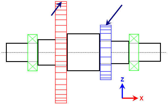
Figure 1: Diagram of Shaft With Gears

Remote Constraint attached to surface of bearing journal with a no-translation constraint at center of bearing (Tx, Ty, and Tz).
Remote Load attached to gear mounting surface with force applied at gear tooth location.
Remote Constraint attached to pinion mounting surface with boundary condition in tangential direction (Ty).
Remote Constraint attached to surface of bearing journal with axial and radial constraint boundary conditions (Ty and Tz).

Figure 2: Equivalent FEA Model Using Remote Loads

Tip: If working with a CAD model, the Mesh CAD Additions Joint command can be used for the bearings to create universal-type joints. The result is the same geometry as created by the remote load command.