Since there is not a single set of values for the contact parameters that will provide an accurate solution for all models, the user must have a good understanding of the functionality of each parameter to determine a proper set of values for the given problem.
You can customize the contact parameters for each pair individually. Select the contact pair in the tree-view, right-click, and choose Settings. Or from the main MES: Surface to Surface Contact dialog box (the spreadsheet), click in the Parameters column for that pair. Either method will access the Controls and Parameters for Contact Pair dialog box. (Any pair whose parameters have been changed will show Custom in the Parameters column. Otherwise, the Parameters column will show Default.)
Controls and Parameters for Contact Pair Dialog Box
Contact problem type
In the Contact problem type drop-down box, select the general type of contact that may occur at any time in the analysis. This selection controls the behavior of the automatic contact stiffness calculation. In some cases, the choice is obvious. In other cases, it may not be clear whether the situation is low speed or high speed. The difference is a matter of solving efficiency. Either selection should give accurate results. The options available are as follows:
- Low Speed Contact (Press-Fit): The contact between the pair is characterized as bringing the parts together slowly (low speed), or the parts are in continuous contact (press fit). The adaptive contact stiffness routine can be used, but is not the default.
- High Speed Contact (Impact): The contact between the pair is characterized as a rapid change occurrence, such as impact or drop test. The adaptive contact stiffness routine will not be used by default.
Contact method
In the Contact method drop-down box, select the method of contact that will be used for the selected contact pair. The options are as follows:
- Frictionless Contact: This contact method will allow parts to experience large relative motion between each other at the contact surfaces. Parts will be able to come into and out of contact throughout the event. No friction will resist the motion between the surfaces. This is the most general contact method.
- Frictional Contact: This contact method is identical to frictionless contact, except that friction can be defined to resist sliding motion between the surfaces. The coefficients that you must define depends on the Friction law setting that you specify in the Modeling Friction section.
- Frictionless Slide / No Bounce Contact: This contact method permits two surfaces to move freely until contact occurs, and then the nodes will not separate, even under tension. The tangential direction can be constrained separately. Use the No slide check box in the Slide / No Bounce Contact Options section to prevent the parts from sliding when they contact; in this case, the contacting parts become bonded. Otherwise, the surfaces are free to slide on each other when the No slide check box is not activated. Note that the surfaces can slide apart if the No slide option is not activated.
- Frictional Slide / No Bounce Contact: This contact type is similar to the slide/no bounce described above. The difference is that friction is included once the surfaces come into contact. Static and sliding friction coefficients can be defined in the Modeling Friction section; see Frictional Contact above for a description. Note: The No bounce checkbox in the Slide / No Bounce contact Options section is always checked and cannot be altered. The No bounce restriction is only applicable when one of the two No Bounce Contact options is selected in the Contact method drop-down box. This checkbox is ignored for the other contact methods.
- Tied Contact: This method is used to simulate bonded contact between surfaces containing unmatched nodes. If this contact method is selected and the surfaces are initially within a specified distance, the surfaces will be considered to be permanently bonded and will not separate nor slide during the event, even under tension. If the distance between the surfaces is greater than the specified distance, contact will not be considered. The specified distance can be controlled using the Tied Contact Options section. If the Tied contact initial interference check box is not activated, the initial distance between the surfaces will be used as the contact distance. If this check box is activated, the distance must be specified in the Tied contact distance field. An analysis using this contact method will not be as fast as an analysis where the nodes on the surfaces are matched. Note: Only the three translations of the nodes (Tx, Ty, Tz) on the surfaces are connected together; the rotations are not connected. Thus, in an arrangement of shell elements projecting out from the face of a brick part - like a cantilever beam made of shells - the shell part will be free to rotate at the brick support if only tied contact is used between the shell and bricks.
Contact type
In the Contact type drop-down box, choose the type of contact that will be used for the selected contact pair.
It is somewhat misleading to describe contact as surface-to-surface. What happens in reality is that the nodes on the second part/surface are connected to the surface of the first part/surface, thereby preventing the nodes from passing through the surface. Optionally, the reverse is true: the nodes on the first part/surface can be connected to the surface of the second part/surface. In no case is the surface of one part prevented from passing through the surface of the second part.
The options for the Contact type are as follows:
- Automatic: The default method will let the processor select between Point to Surface and Surface to Surface contact types based on the contact surface (the mesh) and the material model involved. The processor will also determine which surface will act as the primary surface. (The processor may switch the first and second part/surface before the analysis begins.) However, the Automatic option may not pick the best contact type when large deformation occurs in the analysis. In this case, check the validity of the setup done by the Automatic option; the type of contact selected is listed in the log file (with the list of element count in each part).
- Surface to Surface: This option indicates the contact occurs when the nodes on the secondary part try to pass through the surface of the primary part, and vice versa. The nodes on the primary part can contact the surface of the secondary part.
- Point to Surface: This option indicates the contact occurs when nodes on the secondary part try to pass through the surface of the primary part. The nodes on the primary part/surface can pass through the secondary surface.
- Point to Point: This method is best suited for situations in which the two surfaces experience negligible sliding relative to each other. This option indicates that the contact occurs when the nodes on the secondary part try to pass through the nodes on the primary part; contact between the node and surface of the primary part is not detected. Regardless of how the parts move, the contact force is always between the original pair of nodes connected together. When Point to Point contact is created, the Results environment will show extra parts in the model: one part of Contact elements for each pair of Point to Point contact.
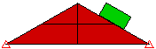
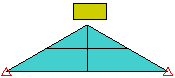
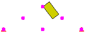
The point to surface method is faster, but you must realize that points on the first part could pass through surfaces on the second part; this contact is not detected. Surface-to-surface contact provides better contact detection, but at the expense of generating more contact elements. It indicates that the nodes on the target part/surface cannot pass through the surface defined by the nodes on the master part/surface (just like point-to-surface contact), and the nodes on the master part/surface cannot pass through the surface on the target part/surface. See Figure 2.
|
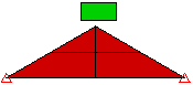
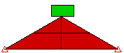
Surface-to-Surface Contact
|
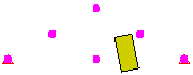
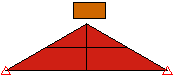
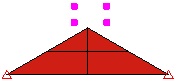
Point-to-Surface Contact (points on the wedge)
|
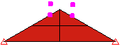
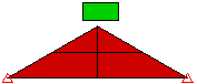
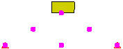
Point-to-Surface Contact (points on the block)
|
|
Time = 0 |
||
|
Equivalent System. The surfaces of both parts are connected through contact. |
Equivalent System. Only the nodes on the wedge exist as far as contact is concerned. |
Equivalent System. Only the nodes on the block exist as far as contact is concerned. |
| Time = 0.024 seconds | ||
|
The surface of the block contacts the surface/node of the wedge. |
The surface of the block contacts the node of the wedge. |
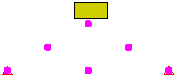
Contact does not occur until the nodes of the block contact the surface of the wedge. The wedge passes through the block. |
| Time = 0.12 seconds | ||
|
The surface of the block slides down the surface of the wedge. |
The block passes in between the nodes of the wedge. |
The block is stuck on the wedge. |
| Time = 0.15 seconds | ||
|
|
|
|
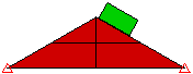
Figure 1: Comparison of Contact Types Three models of dropping a block onto a wedge. Each model uses a different type of contact. |
||
If one of the surfaces in the contact pair is on a part of shell elements, select the side of the shells that will be involved in the contact pair. (The top side is the side opposite of the element normal point defined in the Element Definition dialog box.) Contact only occurs when the two bodies approach from the designated direction. For example, it you indicate that contact occurs with the top of the shell, then contact occurs with the second body is moving in the direction from the top toward the bottom. No contact is made if the second body is moving from the bottom toward the top. Another way to visualize this is as follows: the second object makes contact with the chosen side (either the top or bottom) only when it is approaching from outside the shell. It will not detect contact if it passes through the shell to reach the chosen side. See Figure 3.
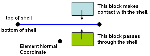
Figure 2: Two Blocks Defined to Contact the Top of the Shell
Contact with line elements (beams, trusses) can only detect contact when the nodes on the line element are contacting the surface of the first part/surface. In addition, specify whether you want all the nodes on the line elements to be considered for contact (All on line element) of only the end nodes (Only those at ends of elements) in the Nodes Making Contact drop-down box. For example, the bristles on a toothbrush made from beam elements only need to have contact from the nodes on the end of the bristles with the teeth; Only those at ends of elements would be used. But a safety net made from truss elements needs to detect contact between all nodes on the net and the falling object; All on line element would be used.
Modeling Friction section
In frictionless contact, the element stiffness matrices are symmetric. Once friction is involved, the matrix becomes asymmetric. Using an asymmetric solver is computationally more expensive than using a symmetric solver. For the sake of efficiency, MES enforces symmetry of element stiffness so that the symmetric solver can be used for frictional contact.
When frictional contact is considered in the analysis, the solution process becomes highly vulnerable from the sliding process. Once the contact surfaces start sliding, the equilibrium state before the sliding is no longer valid and the processor must try to find a new equilibrium state during the solution process. Furthermore, poor convergence is possible due to the symmetry approximation. Each of the available friction law options attempts to control the solution instability in a different manner.
There are three Friction law choices available for nonlinear surface-to-surface contact in Simulation Mechanical:
- Modified Coulomb friction
- Coulomb with viscous friction
- Smooth Coulomb friction
Each of these friction laws, and the parameters that apply to them, are discussed in the subsections that follow.
Modified Coulomb friction
This friction law uses the classical friction algorithm: Coulomb friction. In the basic Coulomb friction model, two contact surfaces can resist shear stress up to a certain amount, determined from friction coefficients and normal contact pressure, before they experience relative sliding motion. The Coulomb friction model is defined as: τ = μP, where μ is the friction coefficient and P is the normal contact pressure. Surface-to-surface contact provides the ability for defining static (μs) and dynamic (μd) friction coefficients. Ideally, once the shear stress exceeds μsP, obtained from the Static friction coefficient input, the two surfaces start sliding. Additionally, the shear stress becomes μdP, where the Sliding friction coefficient value is used.
The ideal situation (no motion until the shear stress exceeds the static value) is difficult to achieve numerically, as described in Figure 3. Thus, a Tangential stiffness ratio is defined when using this friction law. The Tangential stiffness ratio is the ratio of the tangential contact stiffness (Kt) to the contact stiffness in the normal direction (K, set under the Advanced button. See the page Surface-to-Surface Contact Advanced Controls.) A larger tangential stiffness results in better accuracy but at the expense of requiring more iterations. A smaller tangential stiffness provides better convergence (shorter runtime) with the possibility of reduced accuracy. The recommend value is in the range of 0.01 to 1, and the default is 0.01. As the static friction coefficient becomes larger, a smaller tangential stiffness ratio is recommended.
|
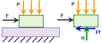
(a) Model and free body diagram of top block. The applied force F is ramped-up over time until it exceeds the static friction force. |
|
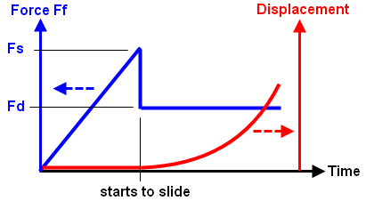
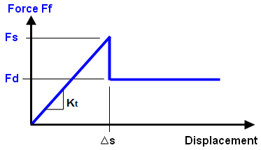
(b) Plot of friction force Ff versus time (blue curve) and displacement versus time (red curve). Until the friction force Ff reaches the limit of static friction (Fs = μs * N), there is no motion of the part. Once the static friction is exceeded, the friction force Ff drops from Fs to Fd (= μd * N), and the part begins to accelerate. |
|
(c) The graphs in (b) are combined to show the friction force versus displacement. Ideally, there is zero displacement until the friction force reaches Fs, and then sliding begins. Numerically, this is difficult to achieve since any displacement other than zero implies a friction force of Fd. |
|
(d) To avoid the numerical instability in (c), the part is allowed to displace a small amount (Δs) while the friction force is less than the static limit (Fs). The amount of motion is controlled by the tangential stiffness (Kt = Fs/Δs). Smaller values of Kt allow the part to displace a larger amount before it starts to slide and are easier to converge, while larger values of Kt (steeper slope) allow less displacement before sliding and are more difficult to converge. The tangential stiffness is calculated by Tangential Stiffness ratio x stiffness in the normal direction. |
| Figure 3: Tangential Stiffness for Modified Coulomb friction |

Coulomb with viscous friction
Unlike the modified Coulomb friction law, static and dynamic coefficients of friction are not both considered in the Coulomb with viscous friction law. In the modified Coulomb friction law, a relatively high force is required to overcome static friction and initiate motion. Once sliding begins, the friction force decreases because the sliding friction coefficient is smaller than the static coefficient. Thus, there is a force discontinuity due to the abrupt change in the friction force. For the Coulomb with viscous friction law, there is no friction force discontinuity when sliding begins. Instead, the friction force gradually increases as the sliding velocity increases.
For the Coulomb with viscous friction option, you must define two parameters:
- Sliding friction coefficient (Fd): This is also referred to as the dynamic friction coefficient. It is the ratio of the tangential force required to maintain relative motion and the normal force between the contacting parts. For example, if it takes 15N of tangential force to keep a block sliding along an adjacent part, and the normal contact force between them is 100N, then the sliding friction coefficient is 15N / 100N = 0.15. For the purpose of this friction law, you should base the sliding friction coefficient on relatively low-speed sliding.
- Viscous friction coefficient (νf): This is the slope of the friction force versus sliding velocity curve. As is true for all viscous effects, the force required to overcome viscous effects is proportional to the speed.
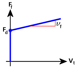
Figure 4: Friction Force versus Sliding Velocity (Coulomb with Viscous Friction)
In Figure 4, the friction force (Ff) curve is defined as follows:
Ff = Fd + νf · Vt
where
Fd is the dynamic (sliding) friction force,
νf is the viscous friction coefficient, and
Vt is the tangential (sliding) velocity between the two parts.
If νf = 0, then Ff = Fd
Smooth Coulomb friction
Like the Coulomb with viscous friction law, the Smooth Coulomb friction law only considers the sliding friction coefficient. This eliminates the friction force discontinuity that occurs between the static and sliding conditions when using the Modified Coulomb friction law. The transition between static and sliding conditions is further stabilized by the inclusion of a smooth transition factor (Φ).
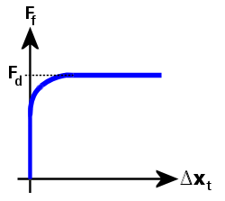
Figure 5: Friction Force versus Tangential Relative Displacement (Smooth Coulomb Friction)
In Figure 5, the friction force (Ff) curve is defined as follows:
Ff = Fd · Φ, and
Φ = tanh(3 · Δxt / δ)
where
Fd is the dynamic (sliding) friction force.
Φ is a transition factor, which makes the friction force smoothly approach zero as the tangential relative displacement approaches zero. Similarly, it makes the friction force smoothly approach the dynamic friction force as the tangential relative displacement increases.
Δxt is the tangential relative displacement, and
δ is a tolerance that is calculated based on the contact stiffness and dynamic friction force.