Gasket materials are used only for the 2D and 3D Gasket elements. This material model is used to model the stress normal to the thickness of a thin gasket-like material. A hypothetical graph of the material response is given in Figure 1. The behavior is defined by the closure (the displacement change of the top and bottom surfaces) and the pressure (normal to the surface).
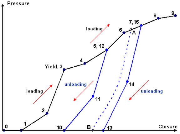
Figure 1: Pressure-Closure Response for Gasket Material
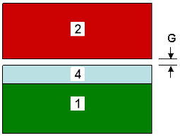
When the gasket is compressed, the pressure increases as a function of closure along the elastic loading curve 0-1-2-3. If the gasket is unloaded before the pressure reaches the yield point 3, it will unload elastically along the curve 3-2-1-0. Segment 0-1 represents the initial gap between the part and the gasket, during which no pressure results. This is a modeling trick: instead of modeling the real gap between the part and gasket, and using surface to surface contact between the part and gasket, the analysis will be faster if the gasket is connected directly to the part and the initial gap is used to simulate the real gap. See Figure 2.
|
|
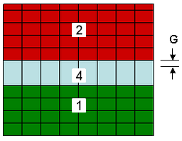
| (a) The physical situation includes an initial gap G between the gasket (part 4) and one of the mating parts (part 2). Surface to surface contact could be used along with the gap between parts 2 and 4, but this would result in a longer analysis run. | (b) In the model, connect part 4 directly to the mating parts (1 and 2) and use the initial gap capability of the gasket material properties to simulate the gap G. Note how the simulated gasket is thicker than the physical gasket. |
| Figure 2: Initial Gap in Gasket Element (The gasket, part 4, is between parts 1 and 2) | |
Point 3 is the user-defined yield point; at higher closures (more compression), the gasket starts to yield and permanent (or plastic) deformation starts to accumulate. Point 7, where the last unloading curve is defined, corresponds to the point that the gasket is fully compressed. Beyond this point, the gasket will behave elastically and no further plastic deformation will result.
When the gasket is unloaded after yielding but before being fully compressed (between points 3 and 7), the unloading behavior is defined by a number of unloading curves (12-11-10, 15-14-13). The user defined unloading curves are interpolated to obtain the actual unloading curve at intermediate position. For example, if the gasket is stressed to point A during an analysis and unloaded, the unloading will follow the dashed line A-B in the figure, where A-B is interpolated from the curves 10-11-12 and 13-14-15. If the gasket is unloaded from a point between the yielding point 3 and the first unloading curve, the interpolation is between loading curve 1-2-3 and unloading curve 10-11-12. If the user does not designate the yielding point, the initial yielding occurs at the first unloading curve.
Reloading of the gasket follows the previous unloading curve (or elastic loading curve if no yielding has occurred), and then continues on the loading curve after passing the new yielding point. In our example, loading the gasket would follow 0-B-A-7-8-9.
If the gasket is loaded beyond the last point, the slope of last segment is used.
Define Gasket Material Properties:
When the material properties for a gasket are entered, either when applying the material properties to a part in a model or in the material library, a default curve with two data points is created.
- To add new points, click the graph at the approximate location and choose Add Point to. This will add a point to the chosen curve (either a loading curve or one of the unloading curves) at the mouse location and place an entry in the Pressure-Closure Curve Data spreadsheet. The precise value can be adjusted in the spreadsheet. New points can also be added to any of the curves by inserting a row in the spreadsheet.
- To delete existing points, either click the graph at the point and choose Delete Point, or select the row in the spreadsheet and click the Delete Row button.
- To add a new unloading curve, click the graph at a point on the loading curve and choose New Unloading Curve. Since the unloading curve must start at a point on the loading curve, be sure to create the point first. Once created, you can add additional points or change the values.
- To delete an unloading curve, click the graph at the first point (the one at 0 pressure) of the unloading curve and choose Delete Unloading Curve. Or, select the first row in the spreadsheet and click the Delete Row button.
- To define the yield point, click the graph at a point on the loading curve and choose Make Yield Point. The yield point is identified on the graph with the symbol (Y) added to the point name. Only points prior to the first unloading curve can be defined as the yield point.
For example, here's how to create the input for the gasket shown in Figure 1. Let's include an initial gap of 0.06 inches, and use the following values based on a 0.1 inch-thick gasket:
| Point | Closure | Pressure | |
|---|---|---|---|
| Loading Cuve | 1 | 0.000 | 0 |
| 2 | 0.008 | 70 | |
| 3 | 0.014 | 250 | |
| 4 | 0.021 | 275 | |
| 5 | 0.028 | 330 | |
| 6 | 0.033 | 400 | |
| 7 | 0.039 | 430 | |
| 8 | 0.044 | 460 | |
| 9 | 0.050 | 470 | |
| Unloading Curve 1 | 10 | 0.014 | 0 |
| 11 | 0.023 | 140 | |
| 12 | 0.028 | 330 | |
| Unloading Curve 2 | 13 | 0.027 | 0 |
| 14 | 0.034 | 200 | |
| 15 | 0.039 | 430 |
- When you create the new material, the default material has just two points: (0, 0) and (1, 1000). If we adjust the last point now, this will set the range of the graph for the material properties. Thus, type the values 0.050 and 470 in the spreadsheet for row (index) 2. Eventually, this will become point 9.
- Add points 2 through 8. Click the graph at the approximate value, and choose Add New Point to Loading Curve. Repeat for each point. (Alternatively, you can place the cursor in row Index 2 and click the Insert Row button 8 times; this will add the new data points and automatically set the values.)
- Adjust the values for the points 2 through 8 by entering the values from the above table into the spreadsheet. The graph will update as each value is entered or when the cursor is moved to a different cell.
- To make point 3 the yield point, click the graph at point 3 and choose Make Yield Point. The point identifier will change from 3 to 3(Y).
- To add the first unloading curve, click the graph at point 5 and choose New Unloading Curve. This will create points 10 and 11, where 11 is forced to be the same values as point 5.
- Adjust the value for point 10 in the spreadsheet to (0.014, 0).
- To add the third point to the unloading curve, click the graph at the approximate location and choose Add Point to Unloading Curve 1. This will create point 11 (and renumber the previous point 11 to point 12).
- Adjust the value for point 11 in the spreadsheet to (0.023, 140).
- To add the second unloading curve, click the graph at point 7 and choose New Unloading Curve. This will create points 13 and 14.
- Adjust the value for point 13 in the spreadsheet to (0.027, 0).
- The third point on unloading curve 2 could be added in the same fashion as above. Click the graph at the approximate location and choose Add Point to Unloading Curve 2. As an alternative, place the cursor in row 14 of the spreadsheet and click the Insert Row button. This will create point 14 (and renumber the previous point 14 to point 15).
- Adjust the value for point 14 in the spreadsheet to (0.034, 200).
- The final step is to account for the 0.06 inch initial gap. Enter the value 0.06 in the Initial Gap field.
Other Inputs
- Stress free reference temperature field: If thermal effects are included in the analysis, enter the stress free reference temperature. This is the temperature at which the gasket in the model experiences no stress due to expansion.
- Thermal expansion coefficient field: If thermal effects are included in the analysis, enter the equivalent thermal coefficient of expansion.
- Initial Gap field: If a gap exists between the part and the gasket, but the mesh of the gasket is connected directly to the part, this value will simulate the gap. The gasket will compress the amount entered in this field without creating any pressure, and then will start to follow the Pressure-Closure curve. The reason for using this input is to create a simpler model. Surface to surface contact could be used between the part and gasket, but this adds complexity to the analysis. See Figure 2 also.