This section discusses the use of Abaqus/Viewer to examine results from the structural analysis generated by Advanced Material Exchange. It is assumed you are familiar with using Abaqus/Viewer to view finite element results and perform any necessary post-processing. This section will focus on results specific to Advanced Material Exchange.
Use Contour Plots to View State Dependent Variables
There are eleven state variables (SDVs) produced by Advanced Material Exchange which can be examined on a contour plot of the model. Review the State Variable Outputs page for a short description of each SDV.
Contour plots are usually the most appropriate means of examining the distribution of the state variables. To generate a contour plot in Abaqus/Viewer, click the contour icon  , or select from the main toolbar. The default variable Abaqus/Viewer plots is the von Mises stress. To view state variables computed by Advanced Material Exchange, open the Field Output dialog box by selecting . State variables (SDV1, SDV2, ..., etc.) are listed within the Field Output dialog box along with more familiar variables such as stress (S) and strain (E). The number of SDVs available in the Field Output dialog box depends entirely on the number of SDVs requested by the Abaqus input file via the *DEPVAR keyword statement
Three of the more useful SDVs are SDV1, SDV9, and SDV11. SDV1 represents the degradation status of the Gauss point locations. A value of 1.0 indicates an undegraded material (no failure). A value of 2.0 indicates the Guass point location has failed and the material stiffnesses have been degraded, allowing failure to progress to the surrounding locations.
SDV9 represents the tangent elastic modulus of the matrix material. When the tangent stiffness decreases, the structure is undergoing plastic deformation, or softening.
SDV11 represents the matrix effective stress. As SDV11 exceeds the maximum effective stress for the von Mises failure criterion, rupture will occur. SDV11 can provide an indication of how close the material is to failure.
Create a Load-Displacement Plot
To detect global structural failure, or to associate a particular distribution of damage with a decrease in overall structural stiffness, we must first examine the relationship between global structural force and global structural deformation. This type of relationship is best examined using a simple 2-D plot of force vs. deformation.
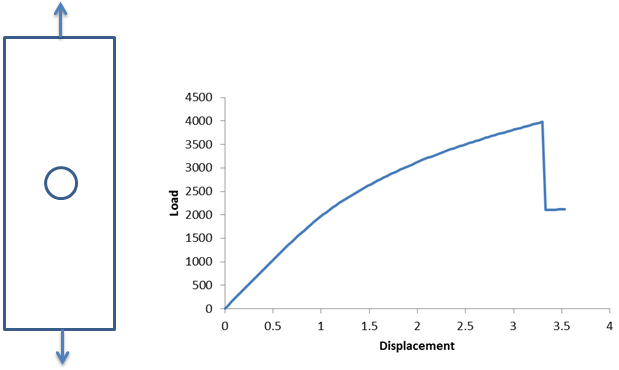
Consider the tensile loaded coupon specimen shown below, machined from an injection-molded plaque. To determine the point in the load history when ultimate failure occurs, we must create a load-displacement curve. By summing the reaction forces on all of the loaded nodes, we can produce the load-displacement plot shown below. We can see a significant amount of plasticity introduced to the structure beginning at a displacement of 1. The plastic deformation continues until we see a large load drop at a displacement of roughly 3.25. This sudden load drop indicates the structure has experienced a catastrophic failure.
If we were to create a contour plot of SDV1 for this model, we would likely see that several elements surrounding the hole have a value of 2.0, indicating catastrophic failure at a displacement of roughly 3.25.