In the steps that follow you will interpret the results of the analysis.
Helius PFA generates several state variable outputs. In this step, a key variable (SV2) is viewed and discussed. SV2 is the state variable that tracks fiber and matrix failure within an element.
To view the composite results in Patran for large models that use solid composite elements, you must open Patran using a special environment variable.
- Type the following in the command prompt to open Patran after the analysis has completed:
>>SET DRANAS_NAST_MEM=2048MB
>>C:\MSC.SOFTWARE\PATRAN_x64\20130\bin\patran.exe -skin
The second line provides the path to the patran.exe file. To determine this path on your machine, right click the Patran 2013 desktop icon and click Properties. - Click File > New and navigate to the directory containing the results. Name the database file Tutorial_1_Nastran_Results.db and click OK.
- Click File > Import and specify the Source as MSC.Nastran Input.
- Navigate to the location of the bulk data file. Click Apply.
- From the Analysis form, set the Action to Access Results and set the Object to Attach Output2.
- Click Select Results File and navigate to the location of the .op2 file. Click OK.
- Click Apply.
- Click the Fringe button on the Results tab.
- Choose the SC1:Step 1, At1:Time = 1 subcase from the Select Result Cases list.
- Select SV2, NonLinear Output from the Select Fringe Result window and click Apply.
The default contour plot uses a results averaging scheme to display results. Set the Averaging Domain to None. This method is more suitable for viewing the discrete values of SV2.
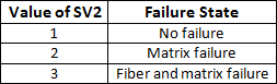
The following table lists three possible values for SV2 and the corresponding failure states. It can be helpful to decrease the spectrum to just 3 colors and specify a user-defined range so the element colors remain consistent. For example, if there are 15 colors in the spectrum and only matrix failure, Patran will automatically adjust the limits to range from 1 to 2 and red elements will correspond to matrix failure but when fiber failure occurs, the range will be adjusted to 1-3 so that red elements correspond to fiber failure instead of matrix failure. By modifying the spectrum and the range of values, SV2 will be always be from 1 to 3.
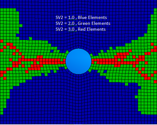
The default ply for the contour plot shown above is Ply 24. To view failure in all of the plies, envelope plots can be used. Envelope plots display the maximum or minimum integration point value across all section points in each element.
- To create an envelope plot, click the Layer button on the Results form and highlight all 24 layers.
- Select Maximum from the menu and click OK. Click Apply on the Results form.
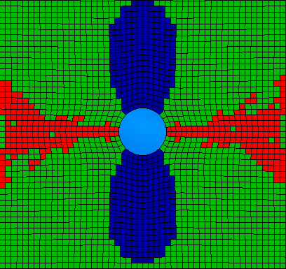
- Starting at the first substep, progress through the load history to view how failure propagates through the coupon.
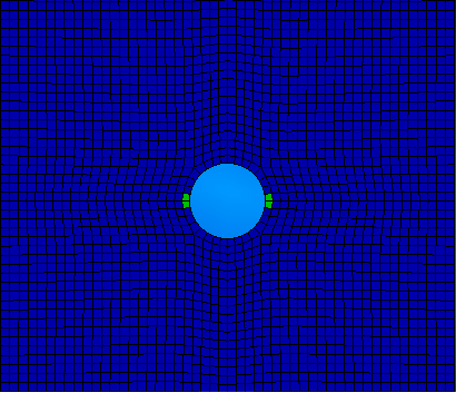
- First matrix failure should occur at time = 0.26 (first image below)
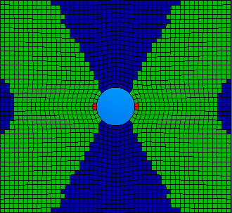
- First fiber failure should occur at time = 0.65 (second image below)
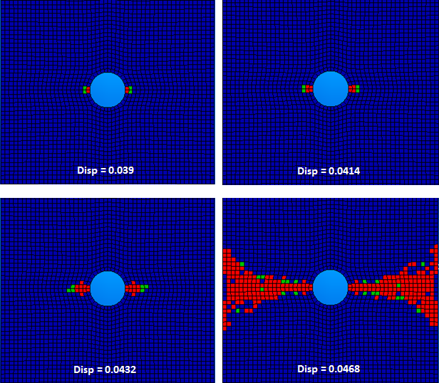
Next, consider the progression of failure in Ply 2, which is one of the main load carrying (0°) plies. The plot below shows failure in Ply 2 at several displacements. As expected, failure initiates at the edges of the notch and progresses laterally towards the edge of the plate until ultimate failure occurs.