Load-displacement plots are commonly used as tools to determine the global stiffness response of a structure. They are particularly useful for progressive failure analyses since they can show how the structure behaves as failure initiates and progresses. We will compare the load-displacement plots for the model with FIBER type element deletion and a model with no element deletion. We will also take a look at two different results in which MATRIX type element deletion was used.
To generate a load-displacement plot, data must be extracted from the output file.
- Select . In the dialog that appears, select the ODB file output option and click Continue.
- In the dialog that appears, select Unique Nodal for the Position and check the RF2 and U2 check boxes. On the Elements/Nodes tab, click Node sets and select LOAD_NODE. Note: Due to the equation constraint defined earlier, the total reaction force can easily be determined from just the load node.
- Click Save, Dismiss, and OK.
- Select . In the dialog that appears, select both sets of data and click OK.
This will generate a text file named abaqus.rpt which contains the load-displacement data we are interested in. We can plot this data with a variety of tools such as Microsoft Office Excel.
The plot below shows four load-displacement curves:
- No ED - Large-notch coupon results without the use of any element deletion criteria
- ED Fiber - Large-notch coupon results with the use of the FIBER type element deletion criteria (model built in this tutorial)
- ED Matrix 0.10 - Large-notch coupon results with the use of the MATRIX RELOAD criteria with a ratio of 0.10
- ED Matrix 0.05 - Large-notch coupon results with the use of the MATRIX RELOAD criteria with a ratio of 0.05
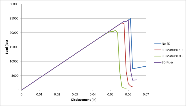
The relation between the individual curves should come as no surprise. The ED Matrix 0.05 model will delete elements in the quickest fashion, therefore we would expect damage to accumulate more quickly and lead to a lower ultimate failure load. The ED Fiber model will delete elements in the slowest fashion, therefore we would expect it to be closest to the No ED model.
We can see as much as a 20% difference in predicted ultimate failure load with these four test cases. This highlights some of the variability that can be achieved with the element deletion controls.
For models in which the damage propagates gradually over several increments we will see a larger discrepancy between the responses with and without the use of element deletion. Until an element has been deleted, it will continue to contribute to the strain energy of the model, and as a result, influence the propagation of damage.