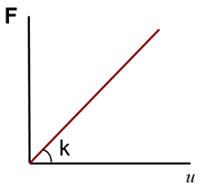
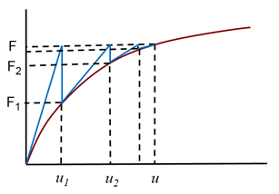
There are many types of behavior that may be referred to as nonlinear. Some examples of nonlinear behavior include displacements which cause loads to alter their distribution or magnitude, materials that change properties as they are loaded, gaps which may open or close. The degree of nonlinearity may be mild or severe.
Linear vs. Nonlinear
The defining line between linear and nonlinear is gray at best. Traditionally, in finite element analysis, there has been a set of criteria that determines if nonlinear effects are important to a particular model. If any of these criteria are present, a nonlinear analysis is needed to accurately simulate real-world behavior. While this criteria still holds true, new capability such as linear contact and new materials such as composites further blur the line on when it is necessary to carry out a full nonlinear analysis.
In Linear static analysis we assume the following:
- Displacements and rotations are small.
- Supports do not settle.
- Materials remains linear, and stress is directly proportional to strain.
- Loads (magnitude, orientation, distribution) remain constant as the structure deforms.
Most problems can usually be considered linear because they are loaded in their linear elastic, small deflection range. For these types of problems, the slight nonlinearity does not affect the results and the difference between a linear and nonlinear solution is negligible.
While many practical problems can be solved using linear analysis, some or all of its inherent assumptions may not be valid:
- Displacements and rotations may become large enough that equilibrium equations must be written for the deformed rather than the original configuration. Large rotations cause pressure loads to change in direction, and also to change in magnitude if there is a change in area to which they are applied.
- Elastic materials may become plastic, or the material may not have a linear stress-strain relation at any stress level.
- Part of the structure may lose stiffness because of buckling or material failure.
- Adjacent parts may make or break contact with the contact area, changing as the loads change.
Thus a Nonlinear effect can be broken down into three main categories:
- Geometric (large displacements)
- Material (plasticity, nonlinear stress-strain curves)
- Boundary condition (loads and constraints, contact interaction)
Note that many problems can exhibit all of these nonlinear effects combined!
The corresponding FEA equations are as follows:
|
Linear Analysis |
Nonlinear Analysis |
|---|---|
|
|
The difference (F – Fi) is called residual force. The process is repeated until F = Fi. |
Where:

The global tangent stiffness matrix  is a function of the global displacements
  because the problem is nonlinear.
The current global displacement vector  is the sum of the preceding
  .
.
Geometric Nonlinearity
The geometric nonlinearity becomes a concern when the part(s) deform such that the small strain assumptions are no longer valid. The large displacements effects are a collection of different nonlinear properties, such as:
- Large deflections
- Stress stiffening/softening
- Snap-thru
- Buckling
- Large strain
The following sections introduce and describe these properties in more details.
Large Deflections
When talking about large deflections we refer to movements or rotations of a part. For instance, if you expect a part to rotate or deflect 45 degrees, then a nonlinear analysis is required. In fact, any rotation more than about 10 degrees will start to have increasing error in a linear analysis. This is because linear analysis assumes small displacement theory in which sin(θ) ≈ (θ).
Stress Stiffening
The stress stiffening effect (sometimes referred to as geometric stiffening) is most pronounced in thin structures where the bending stiffness is very small compared to the axial stiffness. For instance, consider a pre-stiffened drum membrane subjected to a uniform pressure load. The structure is fixed around the perimeter. This thin walled structure will undergo significant stress stiffening as the part transitions from reacting the load in bending, to reacting the load in-plane.
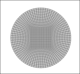
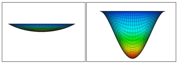
The images below show two results of the pre-stiffened drum membrane. The first image is an actual deflection with large displacement effects turned on (peak deflection is 0.8 inches). The second image is the deformed shape with large displacements turned off. Note in the second image the deformation is scaled down, as the peak deflection is over 5,000 inches.
Another example of stress stiffening is the pitch change on a guitar string as it is tightened. The Young’s Modulus of the guitar string material doesn’t change under tension, but the system stiffens nevertheless.

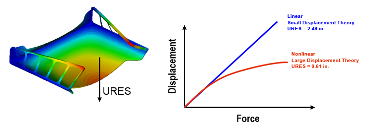
Flat plates under out of plane loading with 3-4 pinned sides are also common stress stiffening cases. In the paper tray shown below, as the distributed load on the face of the part is increased, a linear model predicts a proportional response, whereas the nonlinear model shows that the displacement tapers off as load increases due to the stress stiffening effect.
Note:
- Stress stiffening effects are caused by tensile stresses which result from larger displacements, not by the displacements themselves. The actual displacement in the model is not a clear indication of the degree of nonlinearity, nor is the tensile stress magnitude. A similar tension in one geometry or load orientation may result in significantly less stress stiffening than in another.
- The best way to determine if large displacement effects come into play is by comparing to small displacement results. So run the problem as linear analysis first and then as nonlinear with stress stiffening or large displacement effects accounted for.
- Simplified models can often be used to determine the significance of the displacement effects.
- If small displacement and large displacement results differ ONLY in magnitude, the trends from using small displacement methods will be valid.
Snap-thru and Buckling
Other common geometric nonlinear situations involve snap-thru and buckling problems, often referred to as bi-stable or multi-stable systems. Many snap-thru problems behave nearly linearly until the point where a small amount of additional load causes a large amount of deflection where a secondary stable position is reached. Capturing this snap-thru, or bifurcation, point is a very difficult numerical problem. Once a user has identified that buckling or snap-thru is an issue, a designer can take advantage of the knowledge that FEA solvers may fail in an attempt to model snap-thru and use the solver failure itself to determine at what load buckling is likely to occur.
Large Strain
The large strain effect is nearly always coupled with a nonlinear material model as it involves gross plastic deformation of parts. Cold heading, rubber seal compression, and metal forming are good examples of large strain response.
Material Nonlinearity
There can be a significant difference between the linear and nonlinear material responses, as described in the Nonlinear Materials topic. For any material besides steel, reviewing the stress-strain curves is the best way to understand the nonlinearity of the problem. (Even if you use a linear material model, knowing the nonlinearity is important for interpreting results.)
Simplified models of stress-strain curves are shown below:

A linear model can provide valid data for many materials:
- At low strains
- For trend comparisons
A linear analysis can only predict the onset of yielding. Once the limits of the analysis are exceeded, correlation degrades with the complexity of the stress state.
A nonlinear plasticity analysis can only predict the onset of fracture. The nonlinear material effects can be important when you want to find out what happens past the initial yield of the material.
Alternatively, non-metal materials like rubber and plastic can show a highly nonlinear stress-strain curve even at low strain values. Therefore, getting a more accurate picture of the stiffness of the material through its strain range is important to accurately predicting the stiffness of the overall model.
Brittle materials such as cast iron have little inelastic deformation before failure, so a linear analysis approach for these types of materials is generally okay.
However, the majority of materials and even metals have some amount of ductility. This ductility allows hot-spots to locally yield thus reducing the stresses compared to what a linear analysis would predict.
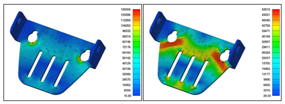
The metal bracket from the image below shows the very different stress distribution between linear and nonlinear materials. The metal has a yield stress of 50ksi. The left image contains the results of a linear material analysis and show peak stresses well above yield. The nonlinear material analysis on the right shows a much different contour due to the stress redistribution. Peak plastic strain was 1% in the nonlinear material analysis.
Boundary Condition Nonlinearity
A model exhibits boundary nonlinearity when the loads, constraints, or load paths change throughout the solution. If the orientation, distribution, or magnitude of applied loads or the load path changes as loading is increased, a nonlinear model may be required. The most common boundary nonlinearities are:
- Contact
- Follower forces
The following sections introduce and describe these properties in more details.
Contact
Contact conditions model the interaction of two separate parts or different surfaces on the same part. Boundary conditions such as surface contact are generally regarded as nonlinear. However, a new trend has emerged lately that allows a contact analysis to run in a linear solution in some FEA applications. In deciding between a linear and nonlinear contact analysis it is best to ask these questions:
- Are there large movements in the model or any of the other nonlinear effects mentioned above?
- Is there significant sliding between contact bodies in the model? Is the contact solution path dependent (for instance a snap-fit)?
- Are detailed contact stresses needed in the model?
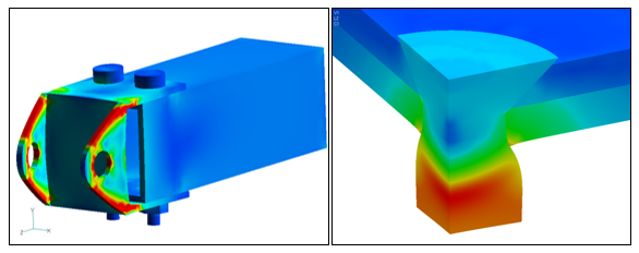
If the answer is yes to any of the three questions above, it is generally recommended to run a nonlinear solution to get the best accuracy. The two models below show two examples of when to use linear contact versus nonlinear. The trailer hitch model on the left, while consisting of 6 parts in an assembly, can be run as a linear contact solution since all the parts are initially in contact and the displacements are small. The rivet model on the right, however, needs a nonlinear solution due to the large displacements involved and the need for a nonlinear plastic material model.
The Surface Contacts topic in the User's Guide contains additional information about contact modeling
Follower Forces
This nonlinear effect simply means that the direction of the forces move with the deformations or movement of the part. Pressure loads are a perfect example of follower forces since they always act normal to a surface. As a part deforms, follower forces will adjust the direction of the loads to ensure they stay normal to the surface.
The cantilevered rectangular beam shown below is loaded with a tip pressure load of 100psi, and three analyses are performed with different large displacement settings (using the LGDISP parameter in Autodesk Nastran In-CAD).
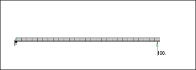
Shown below are the results of the three runs. The first image shows the unrealistic "growth" that occurs when large displacement effects are turned off (LGDISP=OFF). The second image shows the results of large displacements turned on, but follower forces turned off (LGDISP=2). The final image uses large displacement effects with follower forces and is the most accurate (LGDISP=ON).

For more information on how to setup a nonlinear analysis in Autodesk Nastran In-CAD, check out the Nonlinear and Nonlinear Options topics of the User’s Guide.
Nonlinear Element Type
The nonlinear Tension Only Cable element is available in Autodesk Nastran In-CAD.
The tension only cable element is defined as a connector in Autodesk Nastran In-CAD. Right-click on Connectors in the tree and select Edit. Then select Cable for Type (see the Cable Connector topic in the User’s Guide for more details). A material needs to be referenced, along with a cross-sectional area. Either an initial cable tension or an initial cable slack can be specified. For an initial cable tension, the Preload type can be set to Initial in the same dialog box. This setting will treat the initial tension value as a starting preload. This value will be continuously added to the element internal axial load generated from the displacement of the end nodes. The Continuous type setting will force the cable internal load to always be the initial tension regardless of the element nodal displacements. Use of the Continuous setting may result in slower than normal nonlinear iteration convergence.
The cable element must reference a linear isotropic material, but may be temperature dependent. Both thermal and inertial element loads are supported. The cable element, when subjected to lateral loading, requires a small amount of bending stiffness. The default bending stiffness is based on the square of the area of a circular cross-section.
General Guidelines
The following guidelines should be followed when building a nonlinear finite element analysis model:
- Run the analysis as a linear static solution first and make sure the results are as expected.
- Keep the model size small. Simplify the geometry as much as possible before meshing (unnecessary fillets, holes, etc. should be removed). Identify areas of symmetry and cut the model at these planes and apply symmetry boundary conditions. Using symmetry will not only reduce the model size considerably, but the symmetry constraints will help to stabilize the model from rigid body movement.
- Ensure a good quality mesh. The convergence of a nonlinear analysis can be affected by poor quality elements. If the geometry is simple, consider using a mapped plate mesh, or hex mesh for solid elements. Perform distortion checks to make sure there are no severely distorted elements.
- Only apply nonlinear materials in the areas of the model where you expect nonlinear or plastic behavior. This will help to speed up the analysis and can improve the convergence rate.
If surface contact is being used, split up the contact areas into specific regions where you expect contact to occur. Using broad or general surfaces will cause a large number of contact elements to be generated, resulting in an increase in the analysis time.
Troubleshooting
The following steps should be used to diagnose problems when running any nonlinear static analysis:
- Run your model in a linear static solution. Check that the run completed normally and that the results appear correct. Also, check that the Epsilon value is small (< 1.0E-7) and review any warning messages.
- Setup a nonlinear analysis with large displacement effects turned off. Change LGDISP=OFF in the Parameters dialog box under the Nonlinear Solution Processor Parameters section. The Parameters topic of the User's Guide offers some guidance. If PARAM,LGDISP,1 or ON appears in the Model Input File, change this to OFF.
- Turn off any nonlinear materials by commenting out the MATS1 card in the Nastran deck. See the Generate Nastran File topic in the User’s Guide for more details on how to make changes to the Nastran Bulk Data file.
- If the model still does not run after performing steps 2 and 3, go to the nonlinear analysis settings, set the Number of Increments to 1, Output Control to YES, and Maximum Bisections (under the Advanced button) to 1. You should then get 1 output set of results that you can examine to help diagnose the problem in your model.
- If you are able to get the model running as detailed in step 2, turn ON large displacement effects and see if the model still converges. If it does, turn ON the nonlinear material and see if the model converges.
- If, after turning on the nonlinear material your model no longer converges, see the Nonlinear Materials topic for additional info.
If you are getting an E5001: NON-POSITIVE DEFINITE DETECTED AT GRID id COMPONENT n, we recommend you follow the steps listed below to diagnose what is causing the problem:
- Run your model in a linear static solution and make sure it completes and that the results appear correct.
- If it runs okay in linear static, run the model as a nonlinear analysis and use the VIS solver. The VIS solver is chosen in the Parameters dialog box under Program Control Directives – DECOMPMETHOD (see the Parameters topic of the User's Guide). Also change MAXSPARSEITER to 500 iterations to shorten the analysis time. The goal is to force a solution to help diagnose the problem. Unlike all other solvers the VIS will not produce a fatal error for an ill-conditioned stiffness matrix.
- In the Nastran deck on the NLPARM card, change the number of iterations to 1 (field 3) and change the maximum number of iterations to 1 (field 7).
- Run this analysis and look at the results. Please keep in mind this is only a diagnostic run and should not be used as actual results. If you see an area or node with a large amount of displacement/stress, this is the probable cause of the fatal error. This may be caused by badly distorted elements.
|
Previous Topic: Compare the Iterations Exercise |
Next Topic: Flat Walled Tank Exercise |

