Hydrostatic pressure varies linearly from the level of the fluid in the direction of increasing depth of the fluid. The magnitude of the hydrostatic pressure = (fluid density) x (depth below the fluid surface).
You can apply hydrostatic pressure to plate, shell, brick, 3D kinematic, nonlinear membrane, 3D gasket, or tetrahedral elements. By default, the pressure is normal to the face of the elements.
Apply Hydrostatic Pressures
If you have surfaces selected, you can right-click in the display area, select the Add pull-out menu, and choose the Surface Hydrostatic Pressure command. This command is also available on the ribbon (Setup  Loads Hydrostatic Pressure).
To apply a hydrostatic pressure to any supported element type...
- You must specify the weight density (in the Fluid Density field) of the fluid that causes the hydrostatic pressure.
- The hydrostatic pressure can increase along any direction. Specify a point on the top of the fluid in the X, Y, and Z fields in the Point on Fluid Surface section. Only elements below this point receive a pressure.
- Using the Surface Normal of Fluid section, specify a vector that is normal to the surface of the fluid and points into the fluid (that is, in the direction of increasing fluid depth and gravity). When the surface normal is aligned to a global axis, only one of the values for the Point on Fluid Surface is critical.
- For plate elements (linear analyses) and general shell elements (nonlinear analyses), a Side selector is provided within the Creating Surface Hydrostatic Pressure Object dialog box. Choose the Top or Bottom side from the pull-down list. The bottom is the side facing the element normal point, as defined within the Element Definition dialog box. For general shell elements the additional two choices, Both and Neither, are also available from the Side selector. Regardless of whether the load is applied to the top or the bottom surface, the direction is towards the element.
- If you are performing a transient stress (direct integration) analysis or a nonlinear analysis, select the load curve that the pressure follows in the Load Curve field.
Refer to Figure 1 below. Point S represents any point along the top surface of the fluid. The vector V is the direction of increasing fluid depth. The dark red lines are the surface of elements forming a tank. The pressure acting on the wall (Pv) is a function of the depth, increasing linearly as you move downward from the fluid surface. Since the default load direction is normal to the surface of the elements, the pressure along the bottom of the tank acts vertically.
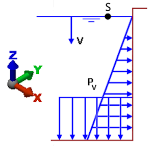
Figure 1: Hydrostatic Pressure
In the Creating Hydrostatic Pressure Object dialog box, there is a Pressure Type option. The choices are as follows:
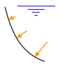
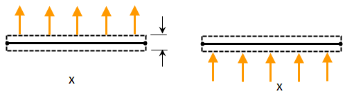
- Normal to the surface: The magnitude of the hydrostatic pressure = (fluid density) x (depth below fluid surface), and the direction is normal to the surface of each plate element. See Figure 2(a) below.
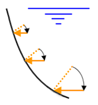
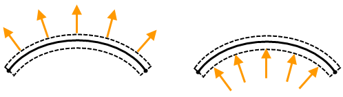
- Full pressure in horizontal: The magnitude of the hydrostatic pressure is calculated as usual, but applied in the horizontal plane. There is no force component parallel to the vector defined by the Surface Normal of Fluid vector. In other words, the direction is normal to the Surface Normal of Fluid, regardless of the slope of the element surfaces. An example of when this option might be used is to simulate the lateral soil pressure acting against an inclined or curved retaining wall. See Figure 2(b) below.
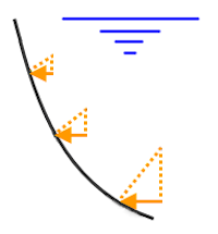
- Horizontal component only: This indicates that only the horizontal component of the hydrostatic pressure is to be applied (vertical component = 0). The magnitude of the pressure = (fluid density) x (depth below fluid surface) x sin(angle between the surface normal direction of the element and the Surface Normal of Fluid vector). The load direction is normal to the Surface Normal of Fluid vector, regardless of the slope of the element surfaces. See Figure 2(c) below.
|
(a) Normal to the surface |
(b) Full pressure in horizontal |
(c) Horizontal component only |
| Figure 2: Types of Hydrostatic Pressure | ||
Visualization of Hydrostatic Pressure Loads:
For CAD-based models, arrows are displayed along surfaces to indicate applied hydrostatic pressure loads in the FEA Editor. The arrows point in the surface normal or horizontal direction (depending upon the load option you select). However, the lengths of the arrows are not scaled to indicate the varying magnitude of the pressure as the fluid depth increases. Arrows are not displayed for elevations above the fluid surface. Therefore, the hydrostatic pressure arrows do not necessarily appear over the entirety of each selected surface.
For non-CAD-based models, H glyphs are displayed along the surfaces in the FEA Editor to indicate hydrostatic pressure loads.
Hydrostatic pressures are converted to nodal forces during the solution phase. For all models, the Results environment displays arrows of varying length, indicating the load direction and the pressure variation at different fluid depths. You can check a model prior to solving it to verify the proper hydrostatic loads.
Notes on General Shell Elements:
Nonlinear General Shell elements take the thickness of the element into account for pressure loading.
(The other planar elements that support hydrostatic pressure loads – plate, membrane, co-rotational shell, and thin shell – consider the pressure to be applied at the midplane. The type of shell element is set using the Element Formulation selector within the Advanced tab of the Element Definition dialog box.)
As mentioned previously, general shell elements have options to apply the hydrostatic pressure to the Top side, Bottom side, Both Sides, or Neither side.
Although the areas of the top and bottom sides of the element are equal in the stress-free condition, large displacement effects can stretch the two surfaces differently. Thus, although uniform pressures of -1000 on the top and 1000 on the bottom may appear to be identical graphically, the results can be different. A similar situation occurs with hydrostatic loads. In addition, for inclined or curved surfaces, taking the thickness into consideration changes the effective fluid depth where the fluid contacts the elements, and therefore affects the hydrostatic pressure (depending upon whether the load is applied to the top or bottom face of the elements). See the figures below.
(a) Planar element, one with a negative pressure applied to the top side of the element (left side of figure) and one with a positive pressure applied to the bottom side of the element (right side of figure). In the stress-free condition, the area of the top side and bottom sides are the same. (The element normal point is indicated by the X.)
(b) As the elements stretch, the area of the top and bottom sides also stretch. Thus, the total force due the same pressure on the top as on the bottom may be different. In this example, the top side stretches more than the bottom side, so the force in the model with the pressure on the top is higher than the force in the model with the pressure on the bottom.
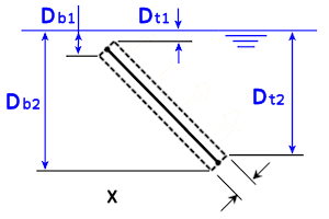
(c) The above image demonstrates how the thickness can affect the hydrostatic pressure for general shell and plate elements. The X represents the element normal point. Notice that the range of fluid depth along the bottom surface (Db1 through Db2) differs from the range of fluid depth for the top surface (Dt1 through Dt2). Therefore, the hydrostatic pressure load will differ depending upon whether it is applied to the top or bottom surface of the planar element. This effect will hold true for general shell elements along inclined, curved, or horizontal surfaces.
Tip: How to Combine Constant and Hydrostatic Pressures
A common occurrence is the combination of a constant pressure (P) and a hydrostatic pressure—for example, a tank partially filled with water and pressurized with air above the water. For 2013 and newer software versions, you can apply multiple surface loads to a single surface, or group of surfaces, in a linear static stress analysis. Apply P as a surface pressure load and add the hydrostatic load to the same surface or surfaces.
However, if you are setting up a nonlinear analysis, or if you anticipate the possibility of both linear and nonlinear analyses (using separate design scenarios, for example), a different method is required. Nonlinear analyses do not support multiple surface loads. There are two methods of applying the combined constant pressure and hydrostatic pressure loads.
- The first method is to specify a free surface point that is at a higher elevation than the actual fluid surface. At the top of the fluid and above, the pressure is P and the applicable equation is...
P = (coordinate of higher free surface - coordinate of actual fluid surface)*(fluid density).
All values are known except for the coordinate of the higher free surface, so calculate this value and enter it for the hydrostatic pressure. Rearranging the terms of the prior equation, solve for the higher free surface as follows:
Coordinate of higher free surface = P / (fluid density) + (coordinate of actual fluid surface)
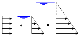
constant pressure + hydrostatic pressure = hydrostatic pressure of greater depth
Naturally, the surface numbers of the model may need to be adjusted so that the hydrostatic pressure is only applied where needed (below the water level) and not in the dotted region of the figure (above the water level). A constant pressure is applied to the surface above the water level. For CAD-based models, splitting the surfaces within the CAD application is the preferred method of doing this, but the surface attributes of the lines can also be changed in Autodesk Simulation.
- The second solution to this problem is to apply a Surface Variable Load. Define an equation, as a function of the appropriate coordinate direction, that will produce the desired linearly increasing pressure. As for the preceding example, the surface of the CAD or FEA model may have to be split to contain the load to the desired region. For more information regarding surface variable loads, refer to the Variable Pressures page.