Frequency Response Analyses

All loads in a Frequency Response analysis are specified within the Analysis Parameters dialog box. Right-click the Analysis Type heading in the browser (tree view) and choose Edit Analysis Parameters, or use the Setup Model Setup Parameters command to access this dialog box.

Parameters Listed at the top of the Frequency Response Analysis Input dialog box

The following three parameters are visible regardless of which dialog box tab is currently displayed:

• Use modal results from Design Scenario: Since the Frequency Response analysis uses the results from a previously run modal analysis, specify which design scenario in the current model contains the modal results.
  Note: The Model Units of the frequency response analysis must be identical to the Model Units of the modal results.
• Cluster Factor for Natural Frequencies: The value in this field is the minimum frequency increase factor (from one mode to the next), for the frequencies to be recognized as separate natural frequencies. For example, value of 0.1 indicates that the successive frequencies need to be 1.1 times higher to consider them as separate modes. This is useful when successive modal frequencies are very close. Use a non-zero cluster factor to ignore essentially duplicate modes. The default value of zero causes all modes to be considered.
• Consider loads of the Same Frequency: When this checkbox is activated, you can specify a Phase Shift for base or nodal excitations listed in the table within the Excited Nodes tab. In this way, you can consider the effects of exciting the model at particular common frequencies (same Frequency index) but with differing phase angles.
  Tip: An example of an application where this option might be needed is the simulation of the harmonic loads from an off-balance motor. Assume that the eccentricity of the mass (center of gravity) at the front of the rotor is in the 12 o'clock direction, and the eccentricity at the back of the rotor is in the 3 o'clock direction. Therefore, both the front and back bearings will experience a harmonic excitation at the same frequency as the rotor spins. However, the phase of the back bearing excitation will lag that of the front bearing by 90 degrees.

Define Exciting Frequencies

The exciting frequencies are defined in the Exciting Frequencies tab of the Frequency Response Analysis Input dialog box. You can create separate sets of exciting frequencies that can be applied to different areas of the model using frequency indices. By default, the frequencies are placed in the frequency index 1 - Freq Index 1. You can create a new frequency index by clicking the (New) button. Specify each of the frequencies in the current frequency index by entering the values in the Frequency (Hz) column. Use the (Delete) button to remove an unwanted frequency index.

Include Natural Frequencies: Activate this check box If you want the natural frequencies to be included as excitation frequencies, in addition to the user-specified frequencies in the table.

Buttons are provided for inserting a row () or deleting a row () in the Exciting Frequencies table. You can also import () or export () a table from/to a CSV file.

Note:

• Specifying multiple frequencies for a given index results in separate load cases. The structure is analyzed as if each frequency occurs independently, and then the square root of the sum of the squares (SRSS response) is calculated.
• In the Results environment, you can view the in-phase, out-of-phase, and SRSS excitations for each frequency. This is controlled by the options in the Results Options Analysis Specific Response Type pull-down menu.

Attention:

• The frequency indices must start with index 1 and be sequential. For example, the indices must be 1, 2 and 3; not 1, 5 and 7.
• All frequency indices must have the same number of forcing frequencies.

Define Excited Nodes

The nodes to which the exciting frequencies are applied are defined in the Excited Nodes tab of the Frequency Response Analysis Input dialog box.

Using the Excited Nodes table, you can use node sets:

• to apply the same frequency index to multiple nodes
• to apply multiple frequency indices to the same node, or
• to apply unique frequency indices to each node set.

To create an additional node set: Click the (New) button. You will be prompted to enter an unused positive integer to define the node set. By default, each node set is named Node Set x (where  x is the integer you specify when creating each new node set).

To rename a node set after it has been created:

• Select the existing node set from the drop-down menu immediately above the table headings.
• Type the new name in the Title field.
• Click Apply.

Attention: The Title input field does not update when you click on different rows of the table. It continues to show the name of the most recently created or renamed node set. The Title field only updates when a node set is selected from the drop-down menu to the left of the Title field.

To delete a node set:

• Choose the node set to delete using the drop-down menu immediately above the Excited Nodes table.
• Click the (Delete) button.

The columns within the Excited Nodes table are defined as follows:

• Column 1 (no heading): This is the index number (a positive integer) that was specified when you created the node set. The first row is always index 1.
• Node Number (Default = Base): For each node set, you can either apply the frequency to a specific node number or to all of the nodes that are constrained by a boundary condition. The latter is known as Base excitation. Node numbers are all positive integers. To apply a load to a specific node, type in the node number (overwriting the word "Base").
  Tip: To determine the node numbers, you must check the model (click Analysis Analysis Check Model). Once the model appears in the Results environment, activate the option Results Options View Show Numbers Node Numbers. You may need to zoom, pan, rotate, change the visual style, or hide selected entities to be able to clearly see the desired node numbers. Record the node numbers of interest for reference when defining the analysis parameters.
• Load Type (Default = Acceleration): The applied load can be specified as a Force Input or Acceleration. (See the Define Amplitudes section below.) A drop-down menu is provided for each cell in this column to choose which of the two types of loads you will specify.
• Load Direction (Default = X Direction): Specify the direction of the applied nodal excitation using the drop-down menu in each cell of this column. Choose either the X Direction, Y Direction, or Z Direction. For excitations applied to specific nodes, the directions correspond to the local coordinate systems to which each node is assigned. For example, the X Direction follows the radial direction for a cylindrical coordinate system. (See the Local Coordinate Systems page for additional details.) For base acceleration, the directions correspond to the global axis directions.
• Frequency Index (Default = 1): Use the drop-down menu in the cells of this column to choose from among the available frequency indices. You must first define additional indices (other than Freq Index 1) within the Exciting Frequencies tab and click Apply to save the settings. Otherwise, the index will not appear in the Frequency Index drop-down menu.
• Scale Factor (Default = 1): This factor multiplies the amplitude of the load applied to the corresponding node set.
• Phase Shift (Degrees) (Default = 0): This value cannot be changed unless the Consider loads of the Same Frequency option (discussed above) has been activated. When this option has been activated, you can type the desired phase shift angle (in degrees) into the cells of this column.
  Caution: Once a phase shift has been defined for any node set, it will continue to be included in the solution, even if the Consider loads of the Same Frequency checkbox is deactivated. To eliminate the phase-shifted excitation, you either have to delete the node set or reset the angle to zero while the Consider loads of the Same Frequency option is enabled.

Note: You can also import () or export () a node set table from/to a CSV file.

Define Damping Ratios

The damping ratios (fraction of critical damping) are defined in the Damping Ratios tab of the Frequency Response Analysis Input dialog box. You create a damping ratio vs. frequency curve by defining data points in the Frequency (Hz) and Damping Ratio columns.

Buttons are provided for inserting a row () or deleting a row () in the Damping Ratios table. You can also import () or export () a table from/to a CSV file.

The damping ratio values at the exciting frequencies (provided in the Exciting Frequencies tab) are calculated by linearly interpolated between the frequency values in the Damping Ratios table. Thus, the frequencies defined in the Damping Ratios tab do not need to match the exciting frequencies.

If any exciting frequency is beyond the range of the smallest to largest frequency entered in the Damping Ratios tab, the amplitude of the closest input frequency is used. Thus, to apply the same load to all exciting frequencies, only one row of input is needed in the Damping Ratios table.

A graph of the damping ratio versus frequency curve is displayed to the right of the table.

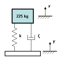
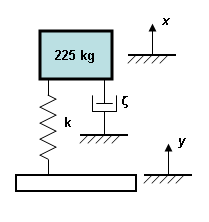
The damping is not specific to a given element. The damping, or equivalent viscous damping, is distributed over the entire model. Thus, the forces due to damping do not appear in the results. For example, the engineering representation of a structure subjected to base acceleration is typically represented as shown in Figure 1a. The force (y) required to move the base includes the damping force z. Since the damping in FEA is viscous damping, a better representation of the analysis is shown in Figure 1b. In this scenario, the damping force does not appear as a result in the analysis. The force reported in the spring k does not include damping.

Figure 1a: Engineering Schematic	Figure 1b: FEA Representation

Define Amplitudes

The amplitudes are defined in the Amplitudes tab of the Frequency Response Analysis Input dialog box. Create an amplitude versus frequency curve by defining data points in the Frequency (Hz) column and either the Acceleration or Force column. The acceleration input unit is g's (1g = standard gravitational acceleration). Values entered into this table are converted to the acceleration units specified in the model unit system. The force input is based on the force units specified in the model unit system.

The acceleration and force values at the exciting frequencies (provided in the Exciting Frequencies tab) are calculated by linearly interpolated between frequency values in the Amplitudes table. Thus, the frequencies defined in the Amplitude tab do not need to match the exciting frequencies.

If any exciting frequency is beyond the range of the smallest to largest frequency entered in the Amplitudes tab, the amplitude of the closest input frequency is used. Thus, to apply the same load to all exciting frequencies, only one row of input is needed in the Amplitudes table.

A graph of the frequency versus amplitudes curve is displayed using a solid green line for acceleration and a dashed blue line for force.

Output Tab

Before the analysis is performed, you can choose to output additional, optional results. Use the following settings in the Output Controls section to indicate which additional results you want to write out:

• Optional data output as text:
  • Activate the Displacement data check box to output the displacement results to the summary file.
  • Activate the Stress data check box to output the stress results to a stress text file.
  Note: The output from these two options can be quite voluminous, and the results available in the Results environment are not affected by these settings. Therefore, if only selected results are needed, it may be better to just use the Results environment. For example, you can select a few nodes of particular interest and save the contents of the Inquire: Results dialog box to a small text file.
• Optional binary output:
  • Activate the Stress/strain at midside nodes (binary) check box to get the stress and strain at midside nodes output to the binary result files. These results can then be displayed in the Results environment. (Midside nodes are an option that can be activated for certain element types using the Element Definition dialog box.)

Percent memory allocation: This setting controls how much of the available RAM is used to read the element data and to assemble the matrices. (When the value is less than or equal to 100%, the available physical memory is used. When the value of this input is greater than 100%, the memory allocation uses available physical and virtual memory.)