A beam element is a slender structural member that offers resistance to forces and bending under applied loads. A beam element differs from a truss element in that a beam resists moments (twisting and bending) at the connections.
These three node elements are formulated in three-dimensional space. The element geometry specifies the first two nodes (I-node and J-node). The third node (K-node) is used to orient each beam element in 3D space (see Figure 1). A maximum of three translational degrees-of-freedom and three rotational degrees-of-freedom are defined for beam elements (see Figure 2). Three orthogonal forces (one axial and two shears) and three orthogonal moments (one torsion and two bending) are calculated at each end of each element. Optionally, the maximum normal stresses produced by combined axial and bending loads are calculated. Uniform inertia loads in three directions, fixed-end forces, and intermediate loads are the basic element based loadings.
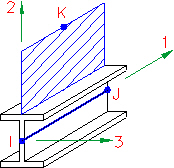
Figure 1: Beam Elements
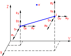
Figure 2: Beam Element Degrees-of-Freedom
For rotation about axes 2 and 3, only the m×R2 effect is considered, where R is the distance from the rotation point to the element. The mass moments of inertia, I2 and I3, are calculated based on the slender rod formula (I2 = I3 = M×L2/12).
The three mass moments of inertia only impact Natural Frequency (Modal) and Natural Frequency (Modal) with Load Stiffening analyses."
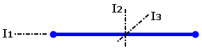
Figure 3: Mass Moment of Inertia Axes
Use Beam Elements When
- The length of the element is much greater than the width or depth.
- The element has constant cross-sectional properties.
- The element must be able to transfer moments.
- The element must be able to handle a load distributed across its length.
Part, Layer, and Surface Properties for Beam Elements
The following table describes what controls the part, layer, and surface properties for beams.
| Part Number | Material properties and stress-free reference temperature |
| Layer Number | Cross-sectional properties |
| Surface Number | Orientation |
Beam Element Orientation
Most beams have a strong axis of bending and a weak axis of bending. Beam members are represented as a line, and a line is an object with no inherent orientation of the cross section. So, there must be a method of specifying the orientation of the strong or weak axis in three-dimensional space. The surface number of the line controls this orientation.
More specifically, the surface number of the line creates a point in space, called the K-node. The two ends of the beam element (the I- and J-nodes) and the K-node form a plane as shown in the following image. The local axes define the beam elements. Axis 1 is from the I-node to the J-node. Axis 2 lies in the plane formed by the I-, J- and K-nodes. Axis 3 is formed by the right-hand rule. With the element axes set, the cross-sectional properties A, Sa2, Sa3, J1, I2, I3, Z2, and Z3 can be entered appropriately in the Element Definition dialog box.
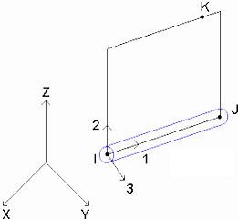
Figure 4: Axis 2 Lies in the Plane of the I-, J-, and K-nodes
For example, the following image shows part of two models, each containing a W10x45 I-beam. Both members have the same physical orientation. The webs are parallel. However, the analyst chose to set the K-node above the beam element in model A and to the side of the beam element in model B. Even though the cross-sectional properties are the same, the moment of inertia about axis 2 (I2) and the moment of inertia about axis 3 (I3) must be entered differently.
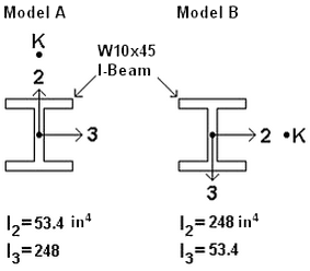
Figure 5: Enter Cross-Sectional Properties Appropriately for Beam Orientations
Default K-Node Location (for Beam Orientation by the Surface Number of the Lines)
Table 1 shows where the K-node occurs for various surface numbers. The first choice location is where the K-node is created provided the I-, J-, and K-nodes form a plane. If the beam element is collinear with the K-node, then a unique plane cannot be formed. In this case, the second choice location is used for that element.
| Table 1: Correlation of Surface Number and K-Node (Axis 2 Orientation) | ||
|---|---|---|
| Surface Number | First Choice K-node Location | Second Choice K-node Location |
| 1 | 1E14 in +Y | 1E14 in -X |
| 2 | 1E14 in +Z | 1E14 in +Y |
| 3 | 1E14 in +X | 1E14 in +Z |
| 4 | 1E14 in -Y | 1E14 in +X |
| 5 | 1E14 in -Z | 1E14 in -Y |
| 6 | 1E14 in -X | 1E14 in -Z |
Notice that the coordinates of the K-nodes are at an extreme distance from the origin. There is a very good reason for this placement. Consider the limited dimensions of any real-world analysis model. The width, length, and height are insignificant as compared to the distance to the K-node location. For example, if +Z is the upward direction, and you use Surface 2 for the floor joists of a 50 meter wide structure. The deviation of the vertical axis of the beams due to them being displaced +/- 25m (or even 50m) from the Z-axis is infinitesimal. Suppose your length unit is millimeters. The Arc Sin of (50,000mm / 1E14mm) is 0.0000000143° (which is zero for all practical purposes). So, you don't have to define multiple K-nodes for vertically oriented beams even when they are positioned at multiple points across a very wide structure.
You can change the surface number, hence the default orientation of the beams. Select the appropriate beam elements (use the Selection Select Lines command) and right-click in the display area. Choose the Edit Attributes command and change the value in the Surface: field.
User-Defined Beam Element Orientation
In some situations, a global K-node location may not be suitable. In this case, select the beam elements in the FEA Editor environment using the Selection Select Lines command and right-click in the display area. Select the Beam Orientations New.. command. Type in the X, Y, and Z coordinates of the K-node for these beams. To select a specific node in the model, click the vertex, or enter the vertex ID in the ID field. A blue circle appears at the specified coordinate. The following image shows an example of a beam orientation that needs the origin defined as the k-node.
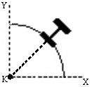
Figure 6: Skewed Beam Orientation
How to Reverse the Direction of Axis 1
The direction of axis 1 can be reversed in the FEA Editor by selecting the elements to change (Selection Select Lines), right-clicking, and choosing Beam Orientations Invert I and J Nodes. This ability is useful for loads that depend on the I and J nodes and for controlling the direction of axis 3. (Recall that axis 3 is formed from the right-hand rule of axes 1 and 2.) If any of the selected elements have a load that depends on the I/J orientation, you choose whether or not to reverse the loads. Since the I and J nodes are being swapped, choose Yes to reverse the input for the load and maintain the current graphical display. The I and J nodes are inverted, and the I/J end with the load is also inverted. Choose No to keep the original input, so an end release for node I switches to the opposite end of the element since the position of the I node is changed.
How to Verify the Correct Axis Orientation
The orientation of the elements can be displayed in the FEA Editor environment using the View Visibility Object Visibility Element Axis commands. The orientation can also be checked in the Results environment using the Results Options View Element Orientations command. Choose to show the Axis 1, Axis 2, and/or Axis 3 using red, green, and blue arrows, respectively. See the following figure.
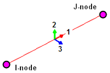
Figure 7: Beam Orientation Symbols (different arrows are used for each axis.)
Specify Cross-Sectional Properties of Beam Elements
The Sectional Properties table in the Cross-Section tab of the Element Definition dialog box is used to define the cross-sectional properties for each layer in the beam element part. A separate row appears in the table for each layer in the part. The sectional property columns are:
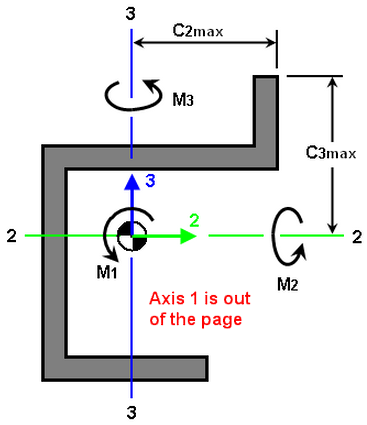
Figure 8: Legend for Defining Cross-Sectional Properties
- A: Specify the cross-sectional area in this column. It is the area of the beam resisting the axial force (δ=FxL/(AxE)). This area must be greater than 0.0.
- J1: Specify the torsional resistance in this column. The torsional resistance is the area moment of inertia resisting the torsional moment M1. The angle of twist within an element is calculated by ϑ=M1xL/(J1xG) where L is the length and G is the shear modulus. For most cross-sections, the torsional resistance is much less than the polar moment of inertia. (For a circular section, J1 equals the polar moment of inertia.) The torsional resistance must be greater than 0.0.
- I2: Specify the area moment of inertia about the local 2 axis in this column. (It is also referred to as I2-2.) The local 2 axis passes through the neutral axis of the cross section and is in the plane formed by the element and the k-node. (See previous paragraph.). The moment of inertia must be greater than 0.0.
- I3: Specify the area moment of inertia about the local 3 axis in this column. (It is also referred to as I3-3.) The local 3 axis passes through the neutral axis of the cross section and forms the right-hand rule with the element (axis 1) and axis 2. The moment of inertia must be greater than 0.0.
- S2: Specify the section modulus about the local 2 axis in this column. The section modulus is calculated from S2=I2/C3max, where C3max is measured parallel to the 3 axis from the neutral axis to the furthermost point on the cross section. This value is not required but is necessary for the bending stress calculation about axis 2 (=M2/S2). If this value is 0.0, the bending stress about the local 2 axis is set to 0.
- S3: Specify the section modulus about the local 3 axis in this column. The section modulus is calculated from S3=I3/C2max, where C2max is measured parallel to the 2 axis from the neutral axis to the furthermost point on the cross section. This value is not required but is necessary for the bending stress calculation about axis 3 (=M3/S3). If this value is 0.0, the bending stress about the local 3 axis is set to 0.
- Sa2: Specify the shear area parallel to the local 2 axis. The shear area is the effective beam cross-sectional area resisting the shear force R2 (shear force parallel to axis 2). If the shear area is 0.0, the shear deflection in the local 2 direction is ignored (usually a safe assumption). The shear area correction is only needed if the beam width is comparable to the beam length.
- Sa3: Specify the shear area parallel to the local 3 axis. The shear area is the effective beam cross-sectional area resisting the shear force R3 (shear force parallel to axis 3). If the shear area is 0.0, the shear deflection in the local 3 direction is ignored (usually a safe assumption). The shear area correction is only needed if the beam width is comparable to the beam length. Note: Hand calculations for the deflection of beams rarely include the effects due to shear within a beam. For example, the well-known equations for the maximum deflection for a cantilever beam and simply supported beam due to a point load (FL3/(3EI) and FL3/(48EI), respectively) only consider the bending effects. If shear effects are included in the finite element analysis by entering values for Sa2 and Sa3, the calculated displacements can be higher than the hand calculations.
For standard cross-sections, or for common shapes with known dimensions, you do not have to enter the individual properties listed above (see the next two sections on this page).
Use Cross-Section Libraries
To use the cross-section libraries, first select the layer for which you want to define the cross-sectional properties. After the layer is selected, click the Cross-Section Libraries button.
How to Select a Cross Section from an Existing Library
- Select the library in the Section database: drop-down menu. Multiple versions of Beam Cross-Section Libraries are provided with the software. (Note: The libraries are set up with IYY (as defined in the AISC manual) corresponding to I2 in the software.)
- Select the cross section type using the Section type pull-down menu. The type designations available for each of the AISC databases are given in Table 5 of the Beam Cross-Section Libraries page. Additionally, you can use the information in Table 2 of the same page to correlate shape designations from non-AISC libraries with the corresponding AISC section types. This table is not comprehensive because the AISC libraries do not contain all of the cross-section types available in some of the non-AISC libraries.
- Select the cross section name in the Section name: list. You can search for a name by typing a string in the field above the list.
- Review the values in the Cross-sectional properties section of the dialog box. If they are acceptable, click OK.
Create a New Library and Add Cross-Sections to a Library
You cannot modify a pre-installed library in any way. However, you can create custom libraries and add user-defined cross-sections to them. You can also copy a library you make at one computer to a new computer and add it to the program. The procedure for creating custom libraries and cross-sections is outlined on the page Create Custom Cross-Section Libraries and Shape Entries.
How to Define Common Shapes
There is a pull-down menu in the upper right corner of the Cross-Section Libraries dialog box that contains a list of common cross-sections. The included shapes are:
- Round
- Pipe
- Rectangular
- Hollow Rectangular
- Wide-Flange Beam
- C Channel
- L-type (angle)
- User-Defined
For all but the last type (User-Defined) you specify the shape by entering the appropriate dimensions. A sketch and data input fields appear after you select a shape. The cross-sectional properties (A, J1, I2, and so on) are calculated for you. Beam elements with these pre-defined shapes can be visualized in 3D within the Results environment.
For User-Defined sections, fill in the data fields in the Cross-sectional properties section in the middle of the dialog box. Sections defined in this manner cannot be visualized in 3D within the Results environment.
- Go to the Element Definition dialog box for the beam part.
- Select a layer (row) in the Sectional Properties table and click the Cross-Section Libraries button.
- Choose the User Defined option from the Section database pull-down menu.
- Select the desired common shape from the pull-down menu in the upper-right corner of the dialog box.
- Alternatively, for cross-sections other than the available common shapes, enter the Cross-sectional properties in the data fields at the center of the dialog box.
- For all but the User Defined option, enter the appropriate dimensions shown at the right side of the dialog box. The cross-sectional properties are calculated and displayed.
- Click OK.
- Repeat steps 2 through 6 for the next layer, or click OK to exit the Element Definition dialog box.
Other Beam Element Parameters
In addition to the cross-sectional properties, the only other parameter for beam elements is the stress free reference temperature. It is specified in Stress Free Reference Temperature field in the Thermal tab of the Element Definition dialog box. This value is used as the reference temperature to calculate element-based loads associated with constraint of thermal growth using the average of the nodal temperatures. The value you enter in the Default nodal temperature field in the Analysis Parameters dialog box determines the global temperatures on nodes that have no specified temperature.
Basic Steps to Use Beam Elements
- Be sure that a unit system is defined.
- Be sure that the model is using a structural analysis type.
- Right-click the Element Type heading for the part that you want to be beam elements..
- Select the Beam option.
- Right-click the Element Definition heading.
- Select the Edit Element Definition command.
- In the Cross Section tab, enter the proper cross- sectional properties for each layer of beams. To use saved properties, common shapes, or standard sections, press the Cross-Section Libraries button. (See the preceding Use Cross-Section Libraries and How to Define Common Shapes sections.
- Once your sectional properties are entered, click OK.