Electrostatic Results

Some of the commands for the Electrostatic Results are identical to the Linear Results. Below are the commands that are unique to electrostatic analyses.

The commands shown in the ribbon depend on the type of electrostatic analysis performed—Field Strength and Voltage or Current and Voltage.

Attention: Due to changes in the software, Electrostatic Field Strength and Voltage results calculated prior to V23.1 (February 2009) should not be used with software versions V23.1 or newer. If these results are needed in V23.1 or newer, the analysis must be performed again.

Voltage

If this option is active, display will be based on the potential at nodes.

Current

This command will only be available for an electrostatic current and voltage analysis. This command will color the model to display the current.

• Magnitude: Sets the display to be based on the magnitude of the current vector. This will always be a positive value.
• X: Sets the display to be based on the dot product of the current vector with a unit vector in the X direction. It shows the component of the total current in the X direction.
• Y: Sets the display to be based on the dot product of the current vector with a unit vector in the Y direction. It shows the component of the total current in the Y direction.
• Z: Sets the display to be based on the dot product of the current vector with a unit vector in the Z direction. It shows the component of the total current in the Z direction.
• Vector Plot: This option will display arrows from the centroid of each elements that will show the magnitude and direction of the current flow through that element.

Rate Through Face

This command will only be available for an electrostatic current and voltage analysis. If this command is active, the display will be based on the current rate normal to the associated face. For brick elements, the face is displayed. To view the inner faces, you should use Results Options View Shrink Elements. A positive value indicates the current is flowing out of the element through the face; negative indicates the current is flowing into the element through the face. For interior elements, the current flowing out of one element and into an adjacent element should be equal. Therefore, the smoothed value should be zero. To see the magnitude of the current flow in this situation, deactivate Results Contours Settings Smooth Results. To sum the current flow through a set of faces, use Results Inquire Inquire Current Results. Select the faces and then select the Sum option in the Summary drop-down box.

Field Lines

This command will only be available for an electrostatic current and voltage analysis. If this command is active, the display will be based on the current field through the model. This will only be available for 2D models when the Invoke Flow Line Generator check box is activated in the Options tab of the Analysis Parameters dialog.

Electric Field

This command will only be available for an electrostatic field strength and voltage analysis. This command will color the model to display the electric field at the centroid of the element.

• Magnitude: Sets the display to be based on the magnitude of the electric field vector. This will always be a positive value.
• X: Sets the display to be based on the dot product of the electric field vector with a unit vector in the X direction. That is, it shows the component of the total electric field in the X direction.
• Y: Sets the display to be based on the dot product of the electric field vector with a unit vector in the Y direction. It shows the component of the total electric field in the X direction.
• Z: Sets the display to be based on the dot product of the electric field vector with a unit vector in the Z direction. It shows the component of the total electric field in the Z direction.
• Vector Plot: This option will display arrows from the centroid of each elements that will show the magnitude and direction of the electric field through that element.
• Field Lines: If this command is active, the display will be based on the electric field through the model. This will only be available for 2D models when the Invoke Flow Line Generator check box is activated in the Options tab of the Analysis Parameters dialog.

Displacement Field

This command will only be available for an electrostatic field strength and voltage analysis. This command will color the model to display the displacement field at the centroid of the element.

• Magnitude: Sets the display to be based on the magnitude of the displacement field vector. This will always be a positive value.
• X: Sets the display to be based on the dot product of the displacement field vector with a unit vector in the X direction. That is, it shows the component of the total displacement field in the X direction.
• Y: Sets the display to be based on the dot product of the displacement field vector with a unit vector in the Y direction. It shows the component of the total displacement field in the Y direction.
• Z: Sets the display to be based on the dot product of the displacement field vector with a unit vector in the Z direction. It shows the component of the total displacement field in the Z direction.
• Vector Plot: This option will display arrows from the centroid of each elements that will show the magnitude and direction of the displacement field through that element.

Tip: Based on the units of the permittivity constant, the units of the displacement field calculation give results in units of current x time/length ² . When the units of the model are Newton, second, meter, ampere, and volt, the results of A-s/m ² are equal to N/(V-m). [You can confirm this by multiplying A-s/m ² by N/N and recalling that a volt is defined as 1 N-m/(A-s).] For other unit systems, the Custom Results can be used to convert the displacement field results to N/(V-m) or any other units of force/(voltage-length) as follows:

1. Convert the existing results to A-s/m2. Recall that this is equal to N/(V-m).
2. Convert N/(V-m) to the units.

Precision

Precision is a method of highlighting stepped changes in results from one element to the next. In an ideal model, the current flux would change smoothly between adjacent element. In the process of discretizing the model with elements, there will always be some change in results from one element to the next. The results are not continuous.

In Electrostatic, the precision is based on the discontinuous current flux magnitude (or electric field) from element to element (across element boundaries). It is calculated as follows:

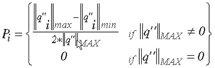
where:

P _i is the precision at node i,

_max is the maximum current flux (or electric field) magnitude at node i obtained by finding the maximum over its neighboring elements,

_min is the minimum current flux (or electric field) magnitude at node i obtained by finding the minimum over its neighboring elements,

_MAX is the global maximum of the current flux (or electric field) magnitude.

Based on the formula, the range of precision values is 0 to 0.5, inclusive.

Electrostatic Force

When the electrostatic forces are generated in a Field Strength and Voltage analysis, Results Contours Voltage and Field Strength will display the electrostatic force at the nodes of the designated surfaces. (See the paragraph Calculating the Forces Caused by the Electrostatic Field in Electrostatic Field Strength and Voltage.)

You can either shade the model based on the magnitude of the electrostatic force, the X, Y, or Z component of the force, or use the Vector plot to display the force using arrows.

Electrostatic Charge

When the charge is generated in a Field Strength and Voltage analysis, Results Contours Voltage and Field Strength Electrostatic Charge will display the electrostatic charge at the nodes of the designated surfaces. The sum of the electrostatic charge on a surface can be used to calculate the capacitance. (See the paragraph Calculating the Forces and Charge Caused by the Electrostatic Field in Electrostatic Field Strength and Voltage.)