A centrifugal load simulates the effect of the entire model spinning about an axis you specify. Only parts with a nonzero material mass density are affected. The model does not actually experience rotation. Rather, the equivalent forces that would occur as a result of angular rotation and/or angular acceleration are calculated and applied to the nodes of each element.
Linear Analyses
Three types of linear analysis support centrifugal loads—Static Stress with Linear Material Models, Natural Frequency (Modal) with Load Stiffening, and Critical Buckling. The model can be spinning at a constant rate and/or can be undergoing a constant angular acceleration rate.
The command implementation is slightly different among the linear analyses. In all three cases, the actual load is defined within the Centrifugal tab of the Analysis Parameters dialog box, and the axes of rotation and angular acceleration can pass through any point is 3D space (that is, the axes do not have to pass through the global coordinate origin). The differences are as follows:
- Static Stress with Linear Material Models:
- The Centrifugal load can be accessed in three ways...
- Right-click the Centrifugal heading under the Analysis Type heading in the browser (tree view) and choose the Edit command.
- Use the ribbon command, Setup
 Loads Centrifugal.
 - Access the Analysis Parameters dialog box (either via the browser or ribbon) and click on the Centrifugal tab.
- Global load case multipliers separately control whether or not the Angular Velocity (Omega) and/or Angular Acceleration (Alpha) loads, as defined within the Centrifugal tab, are active for each load case.
- The axis of angular velocity and the axis of angular acceleration can be separately defined (and can be the same or different).
- The axes or angular velocity and angular acceleration can be along any line in 3D space, as specified via direction vectors.
- The Centrifugal load can be accessed in three ways...
- Natural Frequency (Modal) with Load Stiffening and Critical Buckling:
- The Centrifugal load can be accessed in two ways...
- Use the ribbon command, Setup Loads Centrifugal.
- Access the Analysis Parameters dialog box (either via the browser or ribbon) and click on the Centrifugal tab.
- Use the ribbon command, Setup
- There are no global load case multipliers for the centrifugal load. Rather, it is enabled solely via the Include specified centrifugal load checkbox within the Centrifugal tab of the Analysis Parameters dialog box. If enabled, the centrifugal load affects every resultant mode shape, modal frequency, and buckling multiplier.
- The axis of rotation and angular acceleration must be the same (not separately specified).
- The axis of rotation and angular acceleration must be one of the three global axes (X, Y, or Z).
- The Centrifugal load can be accessed in two ways...
Nonlinear Analyses
Two types of nonlinear analysis support centrifugal loads—MES and Static Stress with Nonlinear Material Models. Load curves control both the rotation speed and the angular acceleration rate over time. The same load curve can be used for both, or you can specify two different load curves for rotation and angular acceleration. The centrifugal load is defined within the Centrifugal tab of the Advanced Analysis Parameters dialog box and can be accessed using one of the following two methods:
- Use the ribbon command, Setup Loads Centrifugal.
- Access the Analysis Parameters dialog box (either via the browser or ribbon), click the Advanced button, and click on the Centrifugal tab.
For either type of nonlinear analysis that supports centrifugal loads...
- The axis of rotation and the axis of angular acceleration can be separately defined (and can be the same or different).
- The axes of rotation and angular acceleration can pass through any point is 3D space (that is, the axes do not have to pass through the global coordinate origin).
- The axes or rotation and angular acceleration can be along any line in 3D space, as specified via direction vectors.
Apply Centrifugal Loads
To apply a centrifugal load to a model...
- Access the appropriate dialog box using one of the methods described above (differs among the various analysis types).
- If included within the dialog box, activate the Include specified centrifugal load checkbox.
- Specify the appropriate magnitudes under Angular Velocity (Omega) and Angular Acceleration (Alpha).
- For nonlinear analyses, select the load curve numbers to use for angular velocity and angular acceleration.
- Specify the axis orientation using one of the methods described above (differs among the various analysis types). For some analysis types, the rotation and angular acceleration axes may be different, and for others, the same axis must be used for both (as detailed above). In addition, some analysis types support non-global axis orientations and others do not (also as detailed above). Use the Point on Axis coordinates and the Direction coordinates or pull-down global axis list to specify the location and direction of the axis (or axes) . The angular rotation follows the right-hand rule about the vector you define.
- For linear static stress analyses, set the Omega and/or Alpha global load case multipliers within the Multipliers tab of the Analysis Parameters dialog box. Tip: A nonzero multiplier is required to activate the load. See the page Analysis Parameters: Static Stress with Linear Material Models.
For example, take the circle centered at the origin in Figure 1. To specify rotation about the Z axis at the origin, enter Point on Axis coordinates of (0,0,0) and Direction coordinates of (0,0,1) - the circle rotates about its center and the center of the circle remains stationary.
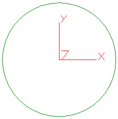
Figure 1: Model 1 Rotating About Origin
However, if you have the circle as shown in Figure 2 centered at (3,0,0) with the same settings for the centrifugal load, the load is based on rotation of the circle about the origin. In other words, the center of the circle moves in a circular path about the global origin. Figure 3 shows a graphical depiction of the path of the circle from Figure 2 under the specified centrifugal load.
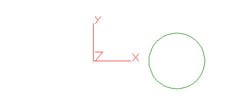
Figure 2: Model 2 – Circle with its Center Not at the Global Origin
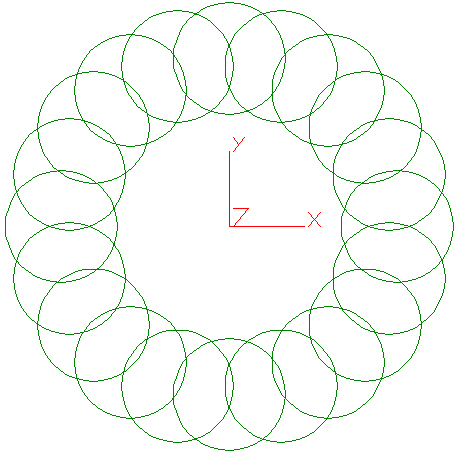
Figure 3: Interpretation of Model 2 Rotating About Origin
- Fully-fix the area or areas of attachment to the supporting shaft or lever.
- Alternatively, constrain tangential motion along the surface of the hole where the rotating parts are fit to the shaft or lever. This constraint takes care of two of the three translational degrees of freedom. In addition, constrain a point, edge, or surface against translation in the axial direction. For example, constrain the area of contact with the shaft shoulder against translation in the normal direction, which prevents axial motion under thrust loads and takes care of the third translational DOF.