Cyclic Symmetry

Cyclic symmetry occurs when the geometry, loads, constraints and results of a partial model can be copied around an axis to give the complete model. A typical example is a fan blade or turbine. If the loads on the blades and geometry repeat, only one blade needs to be modeled instead of the entire hub of X blades. See Figure 1. The result is a smaller analysis which takes less time to analyze.

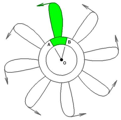
Figure 1: Cyclic Symmetry Example (the highlighted section, including the load, can be copied 7 times about the axis O to create the full model)

In particular, cyclic symmetry forces the radial, tangential, and axial displacements at the nodes on one face (A in Figure 1) to match the same nodes on the opposite face (B in Figure 1).

Note:

• Cyclic symmetry is available only for the analysis types of Static Stress with Linear Material Models, Natural Frequency (Modal), and Transient Stress (Direct Integration). Also, the analysis types that use the modal results (such as Response Spectrum, and so on) produces results that include the effects of the MPCs.
• Cyclic symmetry cannot be used when the results are not cyclic symmetric. This typically occurs in a natural frequency (modal) analysis where some of the mode shapes are cyclic symmetric and some or not. Using cyclic symmetry filters out some of the modes. The same is true for vibration analyses.

Set Up Cyclic Symmetry Models

The basic steps for setting up a cyclic symmetry boundary condition are as follows:

1. Decide where the cyclic symmetry faces is located. Although any cut through the part that results in a cyclic symmetry condition is acceptable, the cut that results in the fewest number of nodes on the cutting faces is generally best. Figure 2 shows some examples. The cut faces do not need to be straight planes, and can have any number of surfaces on the cut face.

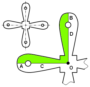
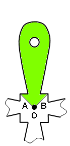
   (a) Option 1. The inset shows the full model. The shaded portion is the model used in cyclic symmetry.	(b) Option 2 results in fewer nodes on the matching opposite cut faces A and B.
   Figure 2: Sample Cut Faces

2. When creating the mesh, the nodes on one face must match the nodes on the opposite face. Another way to think of it is that the nodes from surface A on one face, rotated through X degrees, must match the nodes on surface B of the opposite face. The tolerance used for the node matching is 1% of the shortest line on first part and surface of the defined Matching surfaces (see step 7).
   Tip: Neither the CAD solid mesher nor the 2D mesher forces the meshes on opposite faces to match. If the meshers do not create a matching mesh automatically, you may be able to force them to create a matching mesh by meshing three sections of the cyclic symmetry model. In Figure 2, mesh three blades and then deactivate two of the blades.
3. Apply loads and boundary conditions as normal. The model needs to be statically stable in all six directions, and cyclic symmetry does not prevent motion in the tangential direction --- any amount of rigid-body rotation is an acceptable solution. Normally the part modeled is attached to something not modeled, such as a shaft. In this scenario, the analysis is the displacement of the model relative to the shaft, so the boundary conditions at the attachment to the shaft would be full fixity.
   Tip: Although the cyclic symmetry and applied boundary conditions may produce a statically stable model in theory, the iterative solver can have difficulty converging if the boundary conditions alone do not produce a statically stable model. In this situation, it is recommended to add weak springs to the model. Select a few nodes, right-click, and choose Add Nodal Rigid Boundary. Fix the directions necessary to produce stability, and set the stiffness to a low value. (Low indicates that the loads taken by these weak springs is insignificant compared to the loads applied to the model.)
4. Write down the matching part numbers and surface numbers on the matching opposite cut faces. (In Figure 2(a), it is A to B and C to D.)
5. With nothing selected in the model, right-click in the display area and choose Add Cyclic Symmetry.
6. Enter a Point on axis and Axis direction vector to define the cyclic axis (O in the figures).
7. Use the Add Row button as needed to create as many rows in the Matching surfaces table as there are surface pairs on the cut faces. In Figure 2(a), there are two matching pairs, so the table requires two rows. In Figure 2(b), there is only one matching pair, so the table requires just one row.
8. Enter the part and surface numbers for the matching faces on the cut faces.
9. Click the OK button to save the data.
10. Run the analysis.

Review Results:

Keep in mind that the accuracy of an analysis that uses the iterative solver is dependent on the convergence tolerance. When reviewing the results, one check should be whether the displacements on the opposite faces are identical. This is easier to check if a cylindrical coordinate system is used. See the Local Coordinate Systems page for details.