The concept of controlled chaos is the essence of a particle system. To apply chaos to a Data operator, use the Random suboperator. The Random suboperator generates random values in scalar and vector formats using a variety of algorithms, as described in this section.
Examining Random Examples
Let's start with an example of how to place particles in chaotic manner surrounding a reference object: see included file RandomPositioning.max.

In the data flow illustrated above, the Geometry suboperator (1.) distributes random points uniformly over the surface of a reference object. Its Pair data output is then split off to two different Convert suboperators: Face Local Coordinates (2.) and Compound Index (3.) that includes the face index where a random point is located.
To obtain a desirable volume distribution of particles surrounding the reference object, we need to "lift off" the particles from the surface; this can be done by modifying the Z component of the face local coordinates vector. The Z component is the distance from the face in the direction of the face normal.
A Random suboperator (4.) can be used to define the amount of "lift off." For this example we used Exponential distribution, which is positive and denser around zero. Thus more particles are placed closer to the surface, and the density decreases progressively with the distance from the surface.
Then the modified face local coordinates value and the compound index are converted back into the Pair data format, which is used in the Geometry suboperator (5.) to calculate the particle position in world coordinates.
Let's look closely at the Distribution parameter of the Random suboperator. The parameter defines the type of the random function used in the suboperator. The function type also depends on the data type that Random suboperator produces.
For the next discussion, open the included scene file RandomTemplate.max, which you can use to play with different distribution functions.
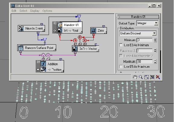
You'll start with a simple distribution type: Uniform Discrete. This is the only type available if the Random suboperator is set to the Integer data type. Discrete is the opposite of Continuous. The Random suboperator generates integer data (in that sense it is discrete) that are uniformly distributed between the Minimum and Maximum values as defined in the UI. In the next example ( RandomTemplate01.max), the Minimum and Maximum values are set to 0 and 30. As a result, you can see that the particle positions are distributed along the lines of X ordinates: 0, 1, 2, 3, etc., up to 30. Here's more about the theory behind Uniform Discrete distribution.
The Real data output type offers the largest variety of available distribution types.
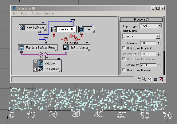
The Uniform distribution type is very similar to Uniform Discrete typethere are Minimum and Maximum values to define the range of distribution, but now the output values are continuously distributed in the range interval. Here's more about Uniform distribution.
The Exponential distribution option is commonly used in reliability engineering. It can be used to model the behavior of units that have a truly random constant failure rate. Another example of exponential distribution is the distribution of individual lifetimes of unstable particles in radioactive decay.
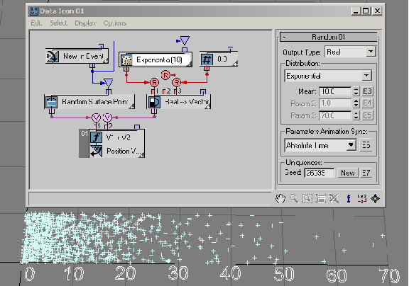
The Exponential distribution option generates positive values only. About half of the generated values are less than the Mean parameter value; with more values generated closer to zero. A generated value can be arbitrary large; however, the larger the value the less likely it is to be generated. In this example ( RandomTemplate02.max), the Mean value is 10; as a result, most of the generated values are between 0 and 70. Here's more about Exponential distribution.
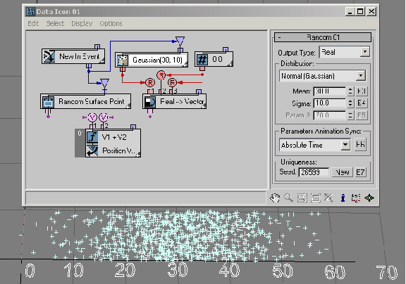
The Normal, or Gaussian, distribution option describes the distribution of independent random errors of observation. Other things that typically take on a normal or close-to-normal distribution include body temperature, shoe sizes, diameters of trees, etc. A normal-distribution graph is a symmetrical, bell-shaped curve. The Mean parameter defines the average value of the generated values (the center of the bell curve), and the Sigma parameter defines how far the generated values can fall out of the average value. The majority of the values (99.7%) are generated inside the 3 Sigma offset interval [Mean3*Sigma, Mean + 3*Sigma]. In the following example ( RandomTemplate03.max) the Mean parameter is 30 with the Sigma parameter set to 10, hence the majority of values generated fall into the interval [0.0, 60]. Normal distribution generates negative and positive values. A generated value can be arbitrary large; however the larger the value the less likely it is to be generated (see the 3 Sigma rule, above). Here's more about Normal distribution.
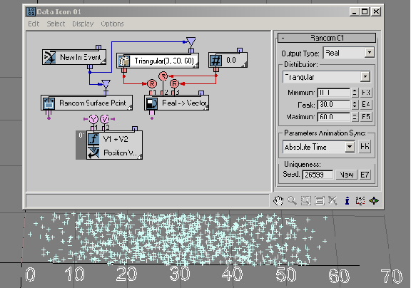
The Triangular distribution option is a simplistic way to describe a random phenomenon that tends to some Peak value and is limited in range by Minimum and Maximum values. In this example ( RandomTemplate04.max), Triangular distribution emulates the Normal distribution from the previous example. Here's more about Triangular distribution.
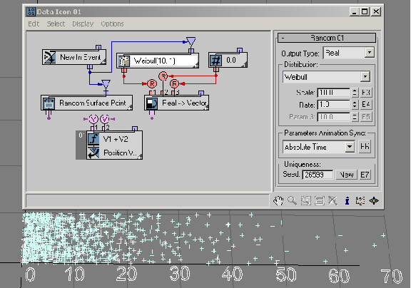
The Weibull distribution method extends Exponential distribution to events that are not purely random; the distribution is commonly used in reliability and lifetime-with-aging modeling. In this example ( RandomTemplate05.max) the Rate parameter is equal to 1.0, thus making the Weibull distribution equal to the Exponential distribution with the Mean parameter as the Weibull Scale parameter.
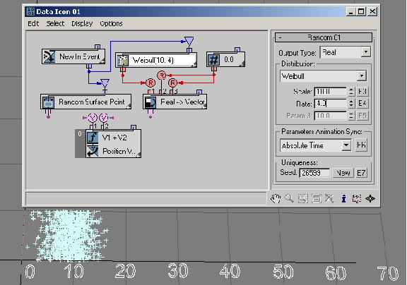
You can use the Weibull distribution to model the time until a given technical device fails. If the failure rate of the device decreases over time, set Rate < 1. If the failure rate of the device increases over time, set Rate > 1. Weibull distribution can also be used to model the distribution of wind speeds at a given location on Earth—every location is characterized by a particular Rate and Scale parameter. In this example ( RandomTemplate06.max), the failure rate is equal to 4 and Scale is equal to 10, making the majority of the random values to be generated in the interval [3.0, 15.0]. Here's more about Weibull distribution.
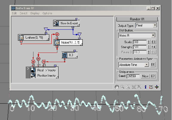
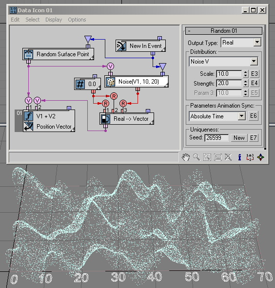
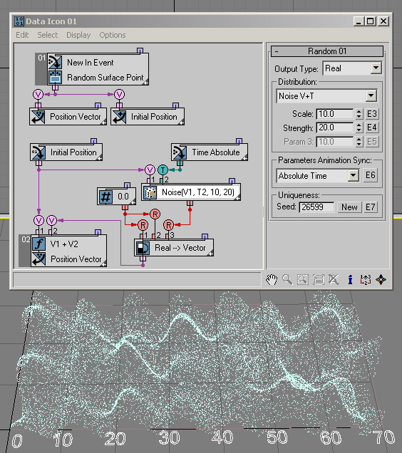
You can use the Noise R, Noise V, Noise V+T, Turbulence V, and Turbulence V+T options to generate pseudo-random noise-type values on the basis of input real, vector and/or time data. The Scale parameter sets the dependency rate between input and output data. Larger values produce smoother noise, lower values more jagged noise. The Strength parameter controls the magnitude of the output values.
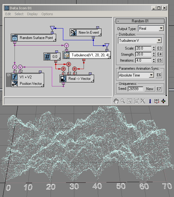
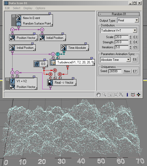
The Turbulence options have an Iterations parameter that controls the number of iterations, or octaves, used to generate the fractal noise. Lower Iterations values create smoother output. The Iterations parameter has range from 1.0 to 10.0. The Noise options generate positive and negative output values; the Turbulence options generate positive values only.
This example ( RandomTemplate07.max) uses a random X coordinate of a particle to generate noise-like random values for the Y coordinate:
In the next example ( RandomTemplate08.max), particles are randomly placed on the surface of the Data Operator icon, and then the position is used as an input for the Random suboperator with the Noise V option. The output data is used to define the particles' heights (Z axis position).
By wiring Absolute Time into the Time input of the ...+T options the generated noise can be easily animated as shown in this example ( RandomTemplate09.max):
The Turbulence options are quite similar to the Noise options. You just need to define the Iterations parameter, as shown in this example ( RandomTemplate10.max).
… and this example ( RandomTemplate11.max):
The last category of distribution options outputs Vector data.
The Uniform distribution option generates random vector values inside a bounding box with limits [–Max X, Max X] for the X component; [–Max Y, Max Y] for the Y component; and [–Max Z, Max Z] for the Z component. With a sufficient number of particles, the bounding box can be filled with random vector points ( RandomTemplate12.max):
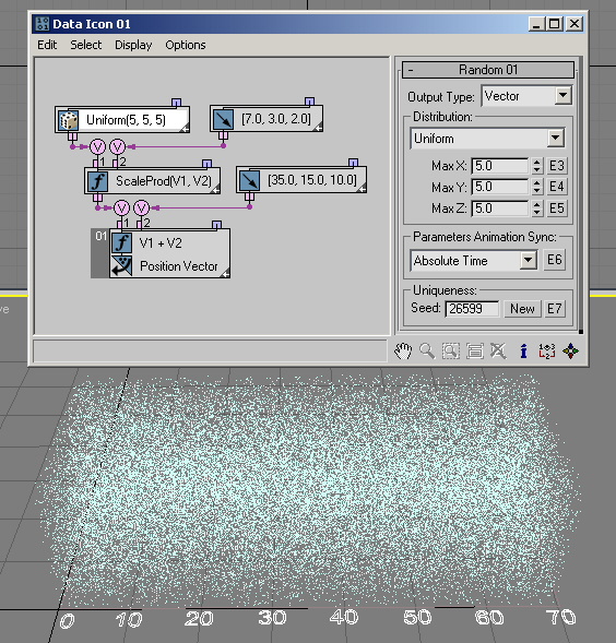
The Sphere Surface option can be used to place particles on the surface of a sphere. However, the most common usage is the generation of a vector with random direction. In this case, the Radius parameter defines the length of the vector ( RandomTemplate13.max):

Or you might want to fill the whole Sphere Volume with random points ( RandomTemplate14.max):
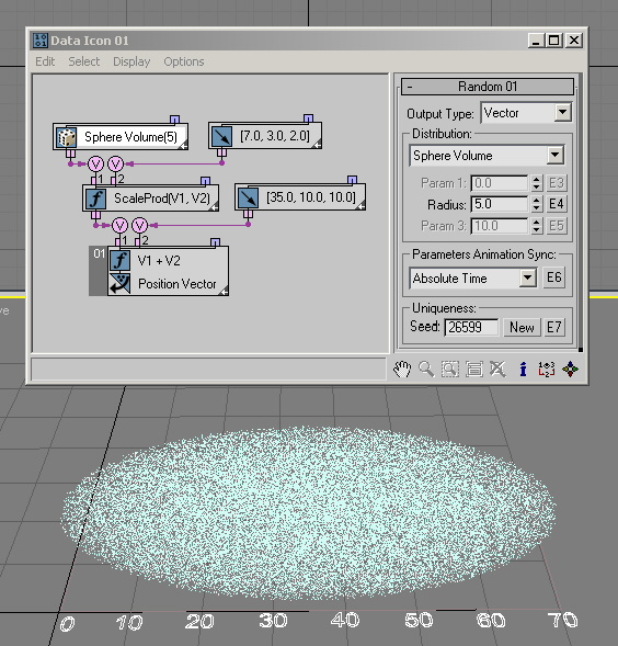
You can use the Normal (Gaussian) option to fill a sphere volume as well, but with this option there is no boundary for the sphere—more points are generated closer to the sphere center, and they diminish outwards. The same 3 Sigma rule as before can be applied here: 99.7% of the points are generated inside a sphere with radius equal to 3*Sigma ( RandomTemplate15.max).
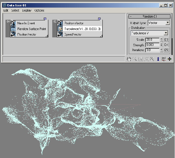
The Noise V, Noise V+T, Turbulence V, and Turbulence V+T options are similar to the Real-data options of the same names, except that they generate Vector data. To illustrate the output data, we can plug it into the Speed channel in Post step, and set speed to zero at Pre step. This way the particles don't go anywhere but we can draw the output as speed lines. In this example ( RandomTemplate16.max) the particles are randomly placed in a rectangle, and then their position is used as an input for the Random suboperator with the Noise V option:
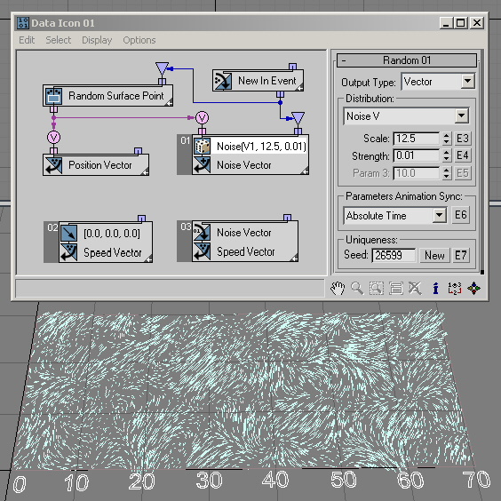
And here ( RandomTemplate17.max) is the same setup, but with the Noise V+T option. We use current time as input for the Random suboperator to have animation for the Noise output:
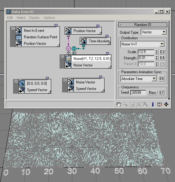
We can wire the Random output into the Speed channel, and use the Position channel as an input for the Random suboperator—it can be used to simulate wind turbulence. This is frame 98 of the scene file RandomTemplate18.max:
Interface
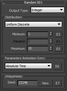
- Output Type
- Choose the data type to output:
- Integer
- Real
- Vector
The Output Type setting determines the parameters available in the Distribution group.
Distribution group
The contents of the Distribution drop-down list are determined by the Output Type choice. The choice of Distribution in turn determines the remaining parameters in the Distribution group.
See the preceding discussion for specific information about the Distribution options and related parameters.
- Parameters Animation Sync
- If you animate the suboperator parameters, the software can begin applying this animation to all particles as of the start frame of the animation or the first frame of the current event, or to each particle based on its age. The options are:
- Absolute Time Any keys set for parameters are applied at the actual frames for which they're set.
- Event Duration Any keys set for parameters are applied to each particle relative to the frame at which it first enters the event.
- Particle Age Any keys set for parameters are applied at the corresponding frames of each particle's existence.
- Particle Lifespan Scales/maps the animation of the parameters onto the particle lifespan period. For example, if a parameter value is animated from 5–20 over frames 0–100, then this parameter has the value 5 when the particle is born, and the value 20 when the particle dies. This way you can, for example, define the change in a particle's scale over its lifespan.
For this option to work properly, there must be a Delete operator set to By Particle Age in the flow to define particle lifespan.
- Time Data Input Adds a Time input to the suboperator, to which you can link any other suboperator that outputs data in Time format.
- E6
- Adds an Equal-type data input for controlling the Animation Sync value. This can receive input only from a Parameter suboperator set to Type=Animation Sync.
- Uniqueness
- Lets you vary the random-number sequence generated by the Random suboperator. Enter a Seed value manually or click New to let the software generate a Seed value.
- E7
- Adds an Equal-type data input for controlling the Uniqueness value. This can receive input only from a Parameter suboperator set to Type=Uniqueness.