After the analysis is complete, open the results with Abaqus/Viewer.
- Click File > Open from the main toolbar in Abaqus and open pedal_assembly_ame.odb. This will open the output database file.
- Click Plot > Contours > On Undeformed Shape to display the contour plot.
- Now select SDV12 from the list of output variables (Result > Field Output). SDV12 represents the strength reduction factor for the weld surface points.
- Display the results for Increment 1 (Step Time = 1E-04 s).
- Click Tools > Display Group > Create and view the Elements by Result value.
- Adjust the Min value to
0 and the Max value to
0.99 and click
Replace.
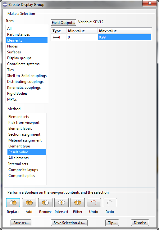
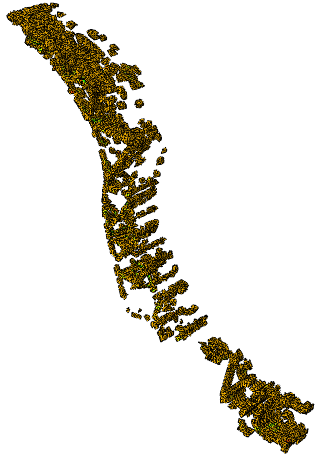
This allows us to view all of the weld surface points in the pedal arm.
The Extron 3019 HS material used in this tutorial was characterized for use with tension and compression. Let's view the compressive response by plotting the S22 component of the stress for one of the elements loaded in compression.
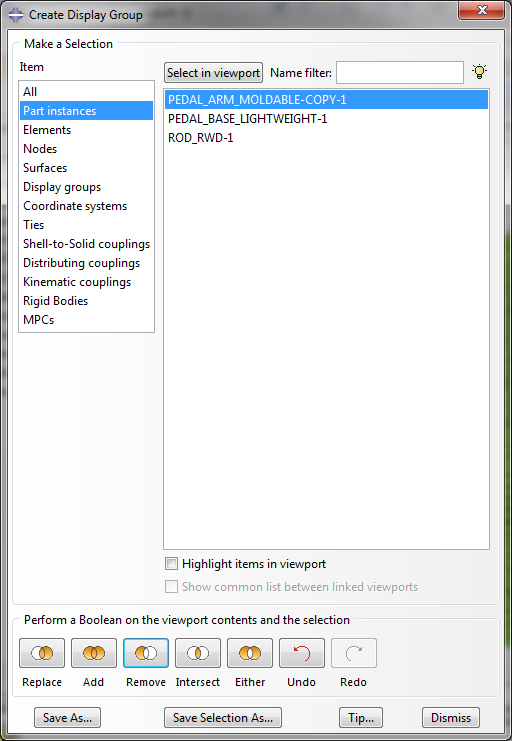
- Create a the Display Group (Tools > Create > Display Group) that hides the pedal arm part instance.
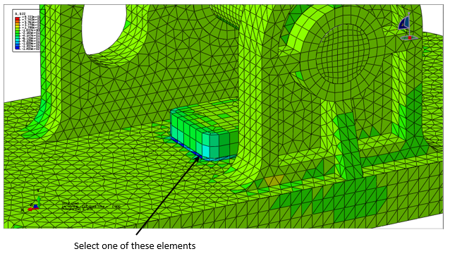
- Now select the S22 component of stress from the list of output variables (Result > Field Output).
- View the results for the last increment in the model (Step Time = 1.00)
- Select one of the elements on the pedal base that is loaded in compression (element 2606 is a good choice) and create an
XY Plot of S22 (Tools > XY Data > Create).
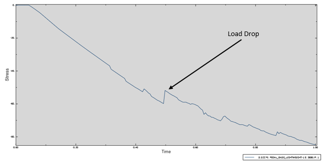
Notice how the element experiences a load drop when the compressive failure criterion is triggered. After the load drop, the plasticity response continues to evolve as before. Since there is still a physical interference between the materials when loaded in compression, this behavior makes sense. Refer to the Compression section of the Theory Manual for more information on how the compressive material model is implemented.