Control the time integration for linear and nonlinear responses of a material.
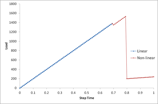
The solution of a progressive failure model can be divided into a linear portion and a non-linear portion. In terms of material nonlinearity, the distinction between the two portions lies in material failure. The linear portion is characterized by the absence of material failure while the nonlinear portion is characterized by the presence of material failure. Ideally, a single increment would be used in the linear portion and many increments would be used in the nonlinear portion to accurately resolve the propagation of damage. With this in mind, it is often the case that a significant portion of the solution is linear. Depending on the incrementation scheme, this can mean that much of the solution time is devoted to solving the linear portion of the solution. For example, consider the load-time plot shown below which color codes the linear and nonlinear portions of the solution for a model with a fixed increment size. Clearly, a majority of the increments are in the linear portion and this time is essentially wasted because the problem is linear until material failure initiates.
To help alleviate this issue, Autodesk has developed a tool to reduce the number of increments the solution spends in the linear portion, while allowing for a fixed increment size in the nonlinear portion. To activate this tool, include the following keyword and data line in the HIN file:
*DAMAGE TIME STEP
DTIME
In practice, the incrementation scheme defined by the *STATIC keyword (in the Abaqus input file) is used during the solution until failure is predicted to occur. Once failure is predicted, Abaqus reverts to the previously converged increment and uses the value specified by DTIME as the increment size. The increment size is allowed to increase until damage occurs and then the increment size is fixed at the value of DTIME. As an example of how this tool is used, consider the following *STATIC and *DAMAGE TIME STEP cards:
Abaqus input file:
*STATIC
0.1, 1.0, 1.0e-05, 0.1
HIN file:
*DAMAGE TIME STEP
0.005
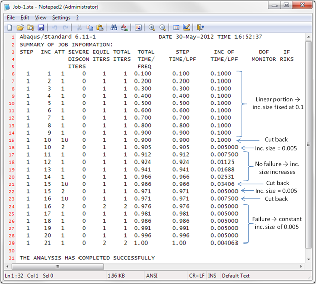
Since the initial and maximum increment sizes are 0.1, the increment size remains fixed at 0.1 until failure is predicted by Helius PFA. When failure is predicted, the solution will cut back to the previously converged increment, then progress using a starting increment size of 0.005. Once failure occurs the increment size will remain at 0.005 for the remainder of the analysis. So instead of using a fixed increment size of 0.005 for the entire solution, a relatively large increment size is used for the linear portion and 0.005 is used for the nonlinear portion. By reducing the number of increments devoted to the linear portion, the overall run time is reduced considerably. The scenario above is demonstrated with the example .sta file shown below.
The *DAMAGE TIME STEP keyword manages material nonlinearity but does not manage other forms of nonlinearity such as contact or geometric nonlinearity. However, since Abaqus manages contact and geometric nonlinearity, there is no conflict and all three forms of nonlinearity can be used with the *DAMAGE TIME STEP keyword.