Plate Elements

What is a Plate Element

Plate elements are three- or four-node elements formulated in three-dimensional space. These elements are used to model and analyze objects (such as pressure vessels) or structures (such as automobile body parts).

The out-of-plane rotational DOF is not considered for plate elements. You can apply the other rotational DOFs and all the translational DOFs as needed.

Nodal forces, nodal moments (except when about an axis normal to the element face), pressures (normal to the element face), acceleration/gravity, centrifugal, and thermal loads are supported. An element Normal Point must be defined in the Element Definition dialog to orient surface normal loads. Since plate elements only have one face, the normal point is required to control the load direction (that is, against which side of the element the load acts). See the Normal Point bullet under The Complete List of Columns that Appear in the Spreadsheet on this page.

Surface loads (pressure, surface force, and so on, but not constraints) and element properties (thickness, element normal point coordinates, and so on) are applied to an entire plate element. Surface loads are based on the CAD surface number or the surface attribute of the lines forming the element. Each element could be composed of lines with four different surface numbers. Therefore, how the surface attribute is applied to the element depends on whether the mesh is created by hand or automatically (by 3D meshing of a CAD model or 2D mesh generation from a sketch). The surface number of the CAD model or the individual lines that form an element are combined as indicated in Table 1 to assign the surface number for the whole element. Loads and properties are then applied based on the surface number of the whole element.

How Mesh Was Created	Definition of Surface Number of Element
Midplane Mesh from CAD Model	All elements coincident with the collapsed (midplane) surface of the CAD model are on the CAD model's surface number, regardless of the surface number of the lines.
Plate/Shell Mesh from CAD Model	All elements coincident with the surface of the CAD model are on the CAD model's surface number, regardless of the surface number of the lines.
2D Mesh from Sketches	All elements are assigned to surface number 1 regardless of the surface number of the lines.
Hand-built Mesh and Modified Automatic Meshes	The highest surface number of any line on the element determines the Surface Number of the entire element. This is referred to as the "voting rule."
Table 1: Definition of Plate Element Surface Number

Note: An automatic mesh that is later modified is treated as a hand-built mesh. Thus, some loads or element properties may change, based on the surface number of the lines, when a CAD-based mesh is modified. Modifications include moving an endpoint of a line; copying or moving a line; deleting a line; or reassigning surface, part, or layer attributes of a line.

Part-Based versus Surface-Based Properties:

Linear plate element properties can be defined on a per-part basis ("Part-based") or a per-surface basis ("Surface-based"). The Surface-based method accommodates plate parts with varying thicknesses or with complex shapes that require more than one element normal point to orient surface normal loads properly. If all of the following conditions are satisfied, part-based properties are acceptable (this is the default option):

The entire plate part has the same thickness, or the midplane thickness determined by the 3D mesher is being used.
A single Normal Point can properly orient all applied surface normal loads, if any are applied.
A single Nodal Order Method and/or Nodal Point definition is suitable for the entire part.
The temperature gradient (delta T thru Thickness), if any, is constant throughout the part.

For each plate part in a model, an Element Options heading appears in the browser. The heading also includes an indication of whether the properties are Part-based or Surface-based. In addition, you can right-click on the Element Options heading and choose Part-based or Surface-based from the context menu to change the option.

(See the Working with Surface-Based Properties page for more information.)

When to Use Plate Elements

Plate elements are suitable under the following conditions:

The thickness is small relative to the length and width (approximately 1/10).
Small displacements and rotations.
Elements remain planar, no significant warpage.
Stress distribution through the thickness is linear.
No rotation about the direction normal to the element.

Plate Element Parameters

To enter the element parameters, select the Element Definition entry in the browser (tree view) for one or more plate element parts, right-click, and choose Edit Element Definition. Alternatively, select the part or parts in the display area or browser, right-click, and choose Edit Element Data.

Note: The Element Definition for multiple parts can be modified simultaneously only if all of the parts are mid-plane meshed, all parts are plate/shell meshed, or all parts are hand-built. You cannot modify parts having a mixture of mesh types at the same time.

Input Included in the Element Definition:

Material Model: Specify the material model for this part in the Material Model drop-down Menu. If the material properties in all directions are identical, select the Isotropic option. If the material properties vary along two orthogonal axes, select the Orthotropic option. (The orientation of the orthotropic axes is then defined using the Nodal Order Method option. See below.)

Element Formulation: Specify which type of element formulation is used for this part in the Element Formulation drop-down menu. The Veubeke option uses the theory by B. Fraeijs de Veubeke for plate formulation for displaced and equilibrium models. This option is recommended for plate elements that have little or no warpage. The Reduced Shear option uses the constant linear strain triangle (CLST) with reduced shear integration and Hsieh, Clough and Tocher (HCT) plate bending element theories. This option is recommended for plate elements that contain significant warpage. The Linear Strain option uses the CLST without reduced shear integration and HCT plate bending element theories. The Constant Strain option uses the constant strain triangle (CST) and HCT plate bending element theories.

Temperature Method: There are three options for performing a thermal stress analysis with plate elements. These are selected in the Temperature Method drop-down menu. If the Stress Free option is selected, the thermal strain (ε) is calculated as the product of the difference of the nodal temperatures (Tnode) applied to the model and the Stress Free Reference Temperature (Tref), and the thermal coefficient of expansion (α): ε = α(Tnode-Tref). The Stress Free Reference Temperature is entered in the appropriate field of the Element Definition dialog. If the Mean option is selected, the thermal strain is calculated as the product of the Mean Temperature Difference (entered in the spreadsheet) and the thermal coefficient of expansion: ε = α(Mean Temperature Difference). If the Nodal dT option is selected, the thermal strain is calculated as the product of the difference of the nodal temperatures applied to the model and 0 degrees and the thermal coefficient of expansion: ε = α(Tnode-0). (Also see delta T thru thickness below.)

Twisting coefficient ratio: The undefined rotational degree of freedom (the direction perpendicular to the element) for a plate element is assigned an artificial stiffness to help stabilize the solution. The magnitude of the artificial stiffness equals the Twisting coefficient ratio times the smallest bending stiffness of the element.

The linear plate element is a combination of planar plate and membrane elements. The rotational degree of freedom perpendicular to the plate element is undefined on a local basis. When combined with other plate elements at an angle, the global rotational degree of freedom is defined. (Visualize this as the in-plane rotation in one element having a component in the out-of-plane direction for the adjacent element.) To avoid a singularity (unknown solution) in the solution of the global stiffness matrix, the twisting coefficient is used to create an artificial stiffness on a local basis. This local stiffness is added to the global stiffness matrix. If this artificial stiffness is too large, the solution behaves as if the model is partially tied down in the twisting direction.

Values for the twisting coefficient ratio that are too large may cause a significant artificial constraint, especially where plates meet at an angle. Values that are too small can increase the maximum/minimum stiffness ratio. A large maximum/minimum stiffness ratio may cause a warning and can make the matrix harder to solve, increasing the chance of an inaccurate solution. (The warning is output during the assembly of the stiffness matrix and before the solving operation. It may be followed by solution warnings which are a much more serious indicator of problems.)

The maximum/minimum stiffness ratio is not always independent of the units. If the maximum and minimum stiffnesses were due to tension, then the units of each (such as N/mm) are canceled. With plate elements, the maximum stiffness is often a tension (units of force/length) and the minimum stiffness is often the out-of-plane rotation (units like force*length/radian), so the maximum stiffness divided by the minimum stiffness does have units. The Twisting coefficient ratio may need to be adjusted depending on the units in use.

Attention: If the Twisting coefficient ratio is too large, some of the applied load is transferred to the ground through the artificial stiffness. In a linear static stress analysis, one way to check if the ratio is affecting the results is to check the reaction forces and moments. If the reactions are less than the applied loads, then some of the load is disappearing through the artificial stiffness. In this case, use a smaller twisting coefficient and rerun the analysis.

Properties: The majority of the Element Definition input is entered in a spreadsheet. The specifics of the input depend on the selection in the Properties drop-down menu and the Use mid-plane mesh thickness check box. The options are as follows:

Properties:
- Part-based: All elements in the part use the same properties regardless of the element's surface number. One row is shown in the spreadsheet.
- Surface-based: All properties in the spreadsheet are entered based on the element's surface number. One row appears in the spreadsheet for each surface number in the part. Some rows may appear because lines exist with the surface number even though no elements have that surface number. The input for such conditions has no effect on the model. (See Table 1 in the previous section What is a Plate Element for the definition of the element's surface number.)
Use mid-plane mesh thickness: This option is available when the part was created from a CAD model by the automatic midplane mesher.
- When activated: The thickness of the elements is determined by the midplane mesher, so the Thickness and Design Variable columns are not shown in the spreadsheet.
- When deactivated: You must specify the thickness of the elements. The Thickness and Design Variable columns are shown in the spreadsheet.

Note: If multiple parts are selected and the Element Definition is modified, the Properties are set to Part-based. If you change the option to Surface-based while editing multiple parts, the surface numbers that appear in all of the selected parts are listed in the spreadsheet. Most likely, some surface numbers will not appear in every part. Be familiar with the model when entering data for multiple parts.

The Complete List of Columns that Appear in the Spreadsheet:

(row selector): This column only appears when the Properties option is set to Surface-based. The checkboxes in the first column are used to select source or target rows when copying and pasting properties, or for editing multiple rows in a single operation. Click the checkbox in the header to alternately select or deselect every row in the spreadsheet with a single click. (See the Working with Surface-Based Properties page for more information.)
Surface: The surface number of the element. Because of the mesh generation method and "voting rule" (see Table 1 under What is a Plate Element above), some surface numbers may appear in the lines of the mesh but may not be the surface number of an element. Some surface numbers listed in the spreadsheet (and the data in their rows) may have no effect on the part. The Surface column is hidden when the Properties option is set to Part-based.
Design Variable: If this check box is activated, then the thickness of the corresponding elements is a variable for design optimization. This column is hidden when Use mid-plane mesh thickness is activated.
Thickness: Enter the thickness of the element. The element is considered to be drawn at the midplane of the thickness the plate element represents. Therefore, half of the entered value for thickness is considered on top of the element while the other half is below the element. Enter a value for the thickness to run the analysis. This column is hidden when the Use mid-plane mesh thickness option is activated.

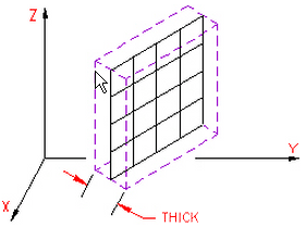
Figure 1: Thickness of a Plate Element

Normal Point X, Y, and Z: A point in space is used to control the orientation of the element's normal axis (local 3 axis), or which side of the element is the "Top" side (+3 side) and which is the "Bottom" side (-3 side). The normal direction is determined by specifying a point in space using the X, Y,, andZ columns under the Normal Point heading. (See Figure 2.) A positive normal pressure is applied normal to the plate elements in the direction of the +3 axis (pushing against the bottom side). A negative normal pressure acts in the opposite direction (pushing against the top side)
As an alternative to typing in the X, Y, and Z coordinates, click the Pick button in the Action column of the Normal Point section to graphically select a point on the model. The Element Definition dialog is temporarily hidden and the cursor is placed in snap-to-vertex mode (as indicated by a padlock icon at the pointer). Then, click the desired normal point and click OK in the Pick Auxiliary Vertex dialog to return to the Element Definition dialog.

Tip: The normal point does not need to be over the element as implied by Figure 2. Mathematically, an infinite plane represents the plate element. The side of the plane that faces the element normal point defines the "Bottom" side of the element.

Figure 2: Determining the Element Normal Orientation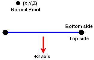
The edge view of the plate element is shown.

Note: The terms "Top" and "Bottom" do not necessarily correspond to the upper and lower surface of a plate element as positioned within a part or assembly. For example, consider a hollow vertical cylinder that serves as a pressure vessel. To apply a normal pressure against the inside surface of the cylinder, you would define the Normal Point in the interior of the vessel. Therefore, the "Bottom" surface would be the inside surface for all elements.

Nodal Order Method: For a general FEA analysis, you can ignore the element's in-plane orientation (axis 1 and 2). The ability to orient elements is useful for elements with orthotropic material models and for easily interpreting stresses in local element coordinate systems. Which method is used to control the in-plane orientation is done with the Nodal Order Method drop-down menu. If the Default option is selected, the edge of an element with the highest surface number is chosen as the ij side. If the Orient I Node option is selected, the node on an element that is closest to the Nodal Point (see next item) is designated as the i node. The j node is the next node on the element following the right-hand rule about the element's normal axis (+3 axis). If the Orient IJ Side option is selected, the side of an element that is closest to the Nodal Point is designated as the ij side. The i and j nodes are assigned so that the j node can be reached by following the right-hand rule about the element's normal axis (+3 axis) along the element from the i node. Once the i and j nodes and axis 3 are defined, the element's local 1 and 2 axes are determined. See Figure 3.

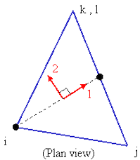
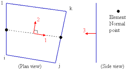
Figure 3: Local 1 and 2 axes for Plate Elements

The dots along the side of the element are at the midpoint of the side.
Nodal Point X, Y, and Z:. If the Nodal Order Method for in-plane orientation is set to Orient I Node or Orient IJ Side, then use these three columns to enter a coordinate defining the element's in-plane orientation (see previous item).
As an alternative to typing in the X, Y, and Z coordinates, click the Pick button in the Action column of the Nodal Point section to graphically select a point on the model. The Element Definition dialog is temporarily hidden and the cursor is placed in snap-to-vertex mode (as indicated by a padlock icon at the pointer). Then, click the desired nodal point and click OK in the Pick Auxiliary Vertex dialog to return to the Element Definition dialog.
delta T thru thickness: Regardless of the method selected in the Temperature Method drop-down menu, you can specify the temperature gradient in the local 3 direction in the delta T thru thickness column. This value is specified on a per-unit-thickness basis. Specifically, the value is equal to the change in temperature across the plate, divided by its thickness:
delta T thru thickness = (T_Top-T_Bottom)/thickness. (See Figure 4.)

This temperature gradient causes the plate to bend but not to grow or shrink.

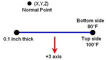
Figure 4: Temperature Gradient Through a Plate Element

ΔT Gradient Through the Thickness:

= (T_Top - T_Bottom) / thickness

= (100 - 80 °F) / (0.1 inch)

= 200 °F/ inch
Mean Temp. Difference: This column only appears when the Mean option is selected from the Temperature Method drop-down menu. The thermal strain in the plate elements is based on the assumption that the difference between the actual temperature and the stress-free temperature is equal to the specified Mean Temp. Difference. The resultant strain is equal to the Mean Temp. Difference times the material's coefficient of thermal expansion. A positive Mean Temp. Difference value causes part expansion, and a negative value causes shrinkage (assuming the coefficient of thermal expansion is positive).

To Use Plate Elements

Ensure that an appropriate unit system is defined.
Ensure that the model is using a linear structural analysis type.
Right-click the Element Type heading for the part that you want to be plate elementsand select the Plate option.
Note: For CAD models meshed using the Midplane or Plate/Shell meshing options, the element type is automatically set to Plate.
Right-click the Element Definition heading.
Select the Edit Element Definition command.
In the Element Definition dialog, select a material model from the Material Model drop-down menu. Select Isotropic if the material properties are independent of direction. Select Orthotropic if the material properties are dependent on direction.
If you are performing a thermal stress analysis, select the method that you want to use for calculating the stress in the Temperature Method drop-down menu. If the Stress Free option is selected, enter an appropriate value in the Stress Free Reference Temperature field. If the Mean option is selected, enter an appropriate value in the Mean Temperature Difference column.
By default, the Properties option is set to Part-based. If you need to assign properties on a per-surface basis, select Surface-based from the Properties drop-down menu. (See the Working with Surface-Based Properties page for more information.)
If the Use mid-plane mesh thickness option is not activated, enter the thickness of the part, or the thickness of each surface.
If you are going to apply a normal pressure load or force to these elements, a Normal Point definition is needed to orient the load. The default Normal Point is 0,0,0. You specify a different point location by entering values in the X, Y, and Z columns of the spreadsheet under the Normal Point heading. A positive pressure load acts against the side of an element that is facing towards this point.
Click OK to accept the properties and exit the Element Definition dialog.