Multipliers
There are two multipliers that control the magnitudes of various electrostatic loads when they are applied to the model. These are located in the General tab of the Analysis Parameters dialog. The value in the Boundary voltage multiplier field multiplies the magnitudes of any applied voltages on the model. The value in the Current or charge sources multiplier field multiplies the magnitudes for any charge or current loads on the model.
A value of zero in any of these fields except for the Boundary voltage multiplier field disables the loads of that type in the model. A value of 0 in the Boundary voltage multiplier field changes the magnitudes of the applied voltages to 0.
Calculate Flow Lines for 2D Models
For 2D models, if the Invoke flow-line generator check box in the Options tab of the Analysis Parameters dialog is activated, the theoretical path of a massless particle through the model are calculated. These results are viewable in the Results environment.
Calculate Forces and Charge Caused by Electrostatic Fields
The forces caused by the electrostatic field can be calculated for individual surfaces of the model (usually a boundary between materials). To calculate these forces, in the Analysis Parameters dialog box, Options tab, activate the Invoke force/charge calculation check box. In the Force/Charge Output table, specify the parts and surfaces for which to calculate the forces . (See the Modify Attributes and Duplicate page for details on changing the part and surface numbers if needed.)
Since the electrostatic force is normally calculated at the boundary between two parts, the part and surface number to specify for the force generator could be on either or both of the bodies in contact (conductor and air, for example). Which surface is correct?
First, decide where to display the force. Then the surface to designate is the part and surface on the mating part in the model. For example, to get the forces to apply to a conductor, use the surface number of the air for the force generator. For the forces to apply to the air, use the surface number from the surface of the conductor.
Since the forces on the matching parts (air and conductor in our example) should be equal and opposite, you may be thinking that which one is chosen for the surface numbers does not matter, provided the direction (positive or negative) is not critical to the analysis. In practice, this is not true. The Coulomb force is sensitive to the change in electric field and the mesh size at the surface. The smaller the mesh, the more accurate the result. The larger the change in electric field, the larger the force. Most bodies have a dielectric constant higher than 1 (air/vacuum), so the change in the electric field is smaller in the body than in the air. A much smaller mesh is required to get accurate forces from the surface of the body compared to the surface of the air.
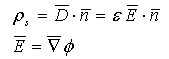
The governing equation for force on conductive surface is as follows:
where the surface integral is carried over the area of the conductive surface and
For a typical element:
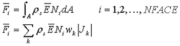
where
ρ s = charge density on the surface
E = electrostatic field
N i , w k , J k = shape and weight functions and Jacobi that give the area
The results of the force generator can be displayed in the Results environment (Results Contours Voltage and Field StrenthElectrostatic Force). Also, the forces can be applied to a stress model to calculate the effect due to the electrostatic forces. See the paragraph
Import Reaction Forces From an Electrostatic Analysis
on the
Forces page.
Voltage and Field StrenthElectrostatic Force). Also, the forces can be applied to a stress model to calculate the effect due to the electrostatic forces. See the paragraph
Import Reaction Forces From an Electrostatic Analysis
on the
Forces page.
The electrostatic charge can be used to calculate the capacitance of a group of conductors if the proper loads are applied. The exterior surface of each conductor must be placed in a unique surface. If a model consists of three conductors, apply voltages of 1V to one of the conductors (the primary conductor) and 0V to the other conductors. In the Results environment, sum the electrostatic charge on the surface of the primary conductor. This is the self-capacitance of that conductor. The sum of the electrostatic charge on each of the remaining two conductors is the mutual capacitance between that conductor and the primary conductor. This process can be repeated using a different primary conductor to create the capacitance matrix.
Solution tab
Solution Options
The type of solver for an electrostatic analysis can be selected in the Analysis Parameters dialog box, Solution tab, in the Type of solver drop-down box. See also Types of Solvers Available for background information. The options available are as follows:
- Automatic If selected, the processor chooses between the Iterative (AMG) and Sparse options based on the model size. The sparse solver is the optimum solver for mid-sized models. The iterative solver is the optimum solver for large models and requires less RAM. If a 64 bit processor is available on the system, the iterative and BCSLIB-EXT solver takes advantage of it.
- Sparse Uses one of two available sparse solvers available in the Type of sparse solver drop-down box. The sparse solvers uses multiple threads/cores when available.
- Iterative (AMG) Uses an iterative scheme to solve the system of equations. The iterative solver uses multiple threads/cores when available.
If for some reason you want to create the solution matrix but not perform the analysis, activate the check box for Stop after stiffness calculations. The only time this is useful is if you must access the equation number matrix. Otherwise, the stiffness matrix is always calculated when running an analysis, so there is no advantage to use this option in normal circumstances.
For the sparse and iterative solvers, the Percent memory allocation field controls how much of the available RAM is used to read the element data and to assemble the matrices. A small value is recommended. (When the value is less than or equal to 100%, the available physical memory is used. When the value of this input is greater than 100%, the memory allocation uses available physical and virtual memory.)
As listed above, some of the solvers take advantage of multiple threads/cores available on the computer. The drop-down Number of threads/cores control is enabled in such situations. You want to use all the threads/cores available for the fastest solution, but might choose to use fewer threads/cores if you need some computing power to run other applications at the same time as the analysis.
Iterative Solver
When chosen, the Iterative Solver section is enabled. The input for this section is as follows:
- Convergence tolerance determines how accurate a solution is found to the matrix of equations. The smaller the tolerance, the more accurate the solution.
-
Maximum number of iterations stops the analysis if the matrix of equations is not solved within this number of iterations.
Attention: The accuracy of the solution depends on the convergence tolerance. A smaller tolerance results in a more accurate solution but can take more iterations. As with any iterative solution, check the results to confirm that they meet the appropriate accuracy. In some cases, performing the analysis twice with a different convergence tolerance is the best way to confirm the accuracy.
Sparse Solver
When chosen, the Sparse Solver section is enabled. The input for this section is as follows:
-
Type of sparse solver lists the sparse solvers currently available. (The sparse solvers are available only for the Windows operating system.) The sparse solvers available are as follows:
- Default Use BCSLIB-EXT solver.
- PVSS Use the Solver Soft sparse solver.
- BCSLIB-EX: Use the Boeing solver. This solver provides a faster solution than the PVSS solver. The BCSLIB-EXT solver can write temporary files to the folder specified by the environment variable USERPROFILE. By default, this variable is set to the folder C:\Documents and Settings\Username where C: is the drive on which the operating system is installed. The error numbers -701 or -804 returned from the BCSLIB-EXT solver means that it ran out of hard disk space for storing the temporary files. If this occurs, change the USERPROFILE variable to a directory that can provide sufficient hard disk space. (See the Windows Help and Support for documentation on changing environment variables.)
- The Solver memory allocation field sets the amount of memory to use during the sparse matrix solution for the BCSLIB-EXT solver. Allocating more memory results in a faster analysis. The other sparse solvers adjust the memory setting automatically; so no setting is required for them.
Control Data in Text Output Files
After the analysis is complete, the analysis results can be output to a text file. In the Analysis Parameters dialog box, Output tab, you can control the data that is output to this file.