Cyclic Symmetry

Cyclic symmetry occurs when the geometry, loads, constraints, and results of a partial model can be copied around an axis to give the complete model. A typical example is a fan or turbine blade. If the loads on the blades and geometry repeat, only one blade needs to be modeled instead of the entire hub and all of the blades. See Figure 1. The result is a smaller analysis which takes less time to solve and consumes much less hard drive space.

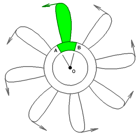
Figure 1: Cyclic Symmetry Example (the highlighted section, including the load, can be copied 7 times about axis O to create the full model)

In particular, cyclic symmetry forces the radial, tangential, and axial displacements at one face (A in Figure 1) to match the displacements on the opposite face (B in Figure 1). The equal displacements are enforced using Multi-Point Constraints (MPCs), which are automatically defined by the software wherever you apply cyclic symmetry.

Note:

• Cyclic symmetry is available only for the following analysis types:
  • Static Stress with Linear Material Models
  • Natural Frequency (Modal)
  • Transient Stress (Direct Integration)
  • Also, linear dynamics analysis types that use the modal results (such as Response Spectrum, Random Vibration, and so on) produce results that include the effects of the cyclic symmetry MPCs.
• Cyclic symmetry cannot be used when the results are not cyclically symmetric. This type of result typically occurs in natural frequency (modal) analyses, where some of the mode shapes are cyclically symmetric and some are not. Using cyclic symmetry filters out some of the valid modes. The same is true for vibration analyses, which are based on modal results.
• In versions of Autodesk Simulation Mechanical prior to 2014, matched (that is, identical) meshes were required at cyclic symmetry faces. That limitation was eliminated in the 2014 release. Cyclic symmetry faces no longer require matched meshes.

Set Up Cyclic Symmetry Models

The basic steps for setting up a cyclic symmetry boundary condition are as follows:

1. Decide where the cyclic symmetry faces are located. The cut faces do not need to be straight planes and can consist of any number of surfaces. Though the meshes do not have to match, the geometry of the symmetry cross sections (area, length, width, and so on) must be the same, except for their rotational position around the axis of symmetry. Although any cut through the part that results in a cyclic symmetry condition is acceptable, the cut that results in the fewest number of nodes on the boundary/cutting faces is generally best. Figure 2 shows two examples.

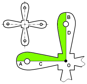
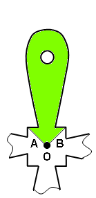
   (a) Option 1. The inset shows the full model. The shaded portion is the model used in cyclic symmetry. Each symmetry plane is comprised of two model surfaces (A and C, for one; B and D for the other).	(b) Option 2 results in a much smaller pair of symmetry faces A and B, and therefore likely a significantly smaller number of nodes along those symmetry faces.
   Figure 2: Sample Cut Faces

2. Apply loads and boundary conditions as you normally do. The model needs to be statically stable in all six directions—three translations and three rotations (when applicable). Cyclic symmetry does not prevent motion in any direction; it merely forces radial, tangential, and axial displacement components on one cyclic symmetry face to be equal to the corresponding components on the matching symmetry face. However, radial rigid-body motion is indirectly impeded due to the fact that the parts would have to stretch or compress circumferentially in order to move radially.

   Frequently, the modeled parts are attached to something not included in the model, such as a shaft or hub. In this scenario, the displacement of the model represents the motion of the part or assembly relative to the shaft or hub. Therefore, the boundary conditions at the attachment to the shaft or hub should provide full fixity.

   Tip: Although the cyclic symmetry and applied boundary conditions may produce a statically stable model in theory, the iterative solver can have difficulty converging if the boundary conditions alone do not produce a statically stable model. In this situation, it is recommended to add weak springs to the model. Select a few nodes, right-click, and choose Add Nodal 3D Spring Supports. Fix the directions necessary to produce stability, and set the stiffness to a low value. (Low is a relative term indicating that the loads taken by these weak springs are insignificant compared to the loads applied to the model.)
3. Write down the part numbers and surface numbers of the matching pairs of cut faces. (In Figure 2(a), it is A to B and C to D.) You cannot select the surfaces graphically while defining cyclic symmetry. In a later step, you will type the part and surface numbers you have recorded into the Cyclic Symmetry dialog.
4. With nothing selected in the model, right-click in the display area and choose Add Cyclic Symmetry.
5. Enter a Point on axis and Axis direction vector to define the cyclic axis (O in the figures). Again, these parameters must be defined numerically. You cannot graphically select vertices or construction points to populate the axis input fields.
6. In the Matching surfaces table, enter the previously recorded part and surface numbers of the pairs of matching symmetry faces. Use the Add Row button as needed to create as many rows as there are surface pairs on the cut faces. In Figure 2(a), there are two matching pairs, so the table requires two rows. In Figure 2(b), there is only one matching pair, so the table requires just one row.
   Note: The numbers in the Matching surfaces table headings (Part 1, Surface 1, Part 2, Surface 2) neither correspond to any actual part or surface numbers nor imply that the part number will necessarily differ between the two faces. They merely label the part and surface number columns that correspond to the first and second cyclic symmetry face, respectively (whatever the specified numbers may be).
7. Click the OK button to save the data.
   Note: No entry is created in the Load and Constraint Groups branch of the browser for Cyclic Symmetry boundary conditions. To verify that the conditions have been applied, revisit the Cyclic Symmetry dialog. The option Include cyclic symmetry in analysis should be activated, and the Point on axis, Axis direction vector, and Matching surfaces parameters should be defined.
8. Run the analysis.

Review Results:

Keep in mind that the accuracy of an analysis that uses the iterative solver is dependent on the convergence tolerance. When reviewing the results, one check should be whether the displacements on the opposite faces are identical. This is easier to check if a cylindrical coordinate system is used. See the Local Coordinate Systems page for details.