Smart bonding is a method of connecting the nodes on adjacent parts even though the meshes do not match. Smart bonding is available for linear and thermal analyses, and it is enabled within the Smart Bonding tab of the General Contact Settings dialog. To access this dialog, double-click the General Contact Settings heading in the browser (tree view), or right-click the heading and choose Edit Settings. The following smart bonding options are available:
- Disable smart bonding
- Coarse bonded to fine mesh
- Fine bonded to coarse mesh
The sections that follow provide guidance for choosing the appropriate smart bonding option.
Smart bonding is designed to connect nodes that are not coincident. A tolerance is required to control how far apart the connected nodes can be. When smart bonding is enabled, double-click a Bonded or Welded contact pair heading in the browser (or right-click the heading and choose Edit Settings) to access the tolerances. You can access the smart bonding tolerance options either from the default contact heading or from an explicitly defined contact pair.
Smart bonding tolerance type: There are two options for the Smart bonding tolerance type, as follows:
- Fraction of mesh size: Uses the input in the Value field times the mesh size to create a dimension. Nodes on the one surface within this distance of the other surface will be bonded. (The mesh size is based on the average element size at the location of the node.)
- Absolute size: Uses the dimension in the Value field for matching the nodes to the adjoining surface.
The software determines which surface nodes are bonded to the adjacent surface based on the relative mesh sizes and the smart bonding mode you specify. This process does not depend on the order of the contact entry shown in the browser. However, the appropriate tolerance value may be affected by the smart bonding mode. The distance between a node on the fine mesh and the nearest node on the coarse mesh may be significantly different from the distance between a node on the coarse mesh and the nearest node on the fine mesh. Hopefully, this concept will become clearer as the difference between the smart bonding modes is further explained.
The smart bonding option applies to Bonded and Welded contact. Other types of contact (except for Free) require the nodes to be matched when using the native Simulation Mechanical (SimMech) solver. See the Types of Contact page for additional information.
- What is referred to as Bonded contact in Autodesk Simulation Mechanical is equivalent to Welded contact in Nastran. Bonding occurs along the entire contact surface for Welded Contact when using the Nastran solver. This behavior differs from Welded Contact when using the SimMech solver, in which case only the perimeter of the contacting surfaces is bonded (simulating the effect of a weld bead around the perimeter of the part interface).
- Do not use smart bonding if the same mesh will be used for another analysis, and if the other analysis does not support smart bonding (such as a nonlinear analysis when using Welded contact). Also, if the contact type will be changed to a type that does not support smart bonding (such as from Bonded to Surface contact), then the meshes should be matched for both analyses.
Smart Bonding Function
Smart bonding transmits loads from the nodes on one part to the adjacent nodes on the other part by using equations to link the degrees of freedom of the parts together (displacements for stress analysis, temperature for heat transfer). This linking is done with the same method as Multi-Point Constraints (MPCs). In stress analysis, the translations are linked for brick and 2D elements. For plate to plate elements, the translations and rotations are linked. See Figure 1 for examples.
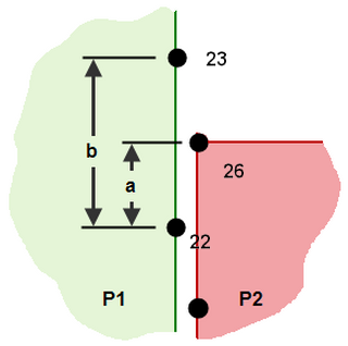
Consider a contact pair between Part A/Surface C and Part B/Surface D. Since the nodes on surface D may be connected to nodes on surface B that exist outside the area of surface D, the smart bonding can distribute the load from Part C to Part A over a larger area than the physical contact area. Naturally, the degree that the load is spread out depends on the size of the mesh. See Figure 1(a).
|
TX26 = TX22 + (a/b)(TX23-TX22) TY26 = TY22 + (a/b)(TY23-TY22) TZ26 = TZ22 + (a/b)(TZ23-TZ22) T is translation in X, Y, or Z at indicated node. |
|
(a) Solid (P1) to solid (P2) connection with smart bonding, stress analysis. Since part 2 is connected to part 1 at nodes 22 and 23, the load is transferred over a larger area than the interface between parts 1 and 2. This approximation is more accurate as the mesh size on part 1 is reduced. |
|
|
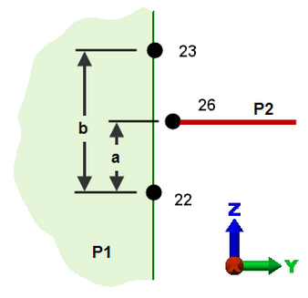
TY26 = TY22 + (a/b)(TY23-TY22) TZ26 = TZ22 + (a/b)(TZ23-TZ22) RX26 = 0 R is rotation about X, Y, or Z at indicated node. |
|
(b) Plate (P2) to solid (P1) connection with smart bonding, stress analysis. (2D view considered for simplicity) |
|
|
|
T26 = T22 + (a/b)(T23 - T22) T is the temperature at the indicated node. |
| (c) Solid to solid connection with smart bonding, heat transfer analysis. | |
| Figure 1: Smart Bonding Examples | |
Tip Concerning Midside Nodes
Use smart bonding to connect the midside nodes on part A (a part where more accurate results are desired) with the corner nodes on part B (a part without midside nodes, not requiring as high of accuracy).
|
|
| Without smart bonding, the midside nodes in the part on the right can pull away from the face of the left part. (Only nodes on contact face shown for clarity.) | With smart bonding, the midside nodes are bonded to the face of the left part. Thus, the midside nodes cannot pull away. (Parts shown with slight gap for clarity.) |
| Figure 2: Bonding Midside Nodes | |
Note Concerning Legacy Models
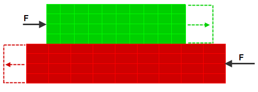
Models created prior to the introduction of smart bonding may have relied on an un-matched mesh to create free surfaces even though the contact type was set to bonded. If such models are re-analyzed, the smart bonding should not be enabled; otherwise, such surfaces will now behave as bonded. See Figure 3. (By default, smart bonding is disabled for legacy models.)
|
(a) Prior to smart bonding, parts are not bonded because the nodes do not match. (Actually, no type of contact would have worked since the nodes do not match.) A tangential force F causes the parts can separate. |
|
(b) If the same model is opened in software with smart bonding capability, and if the contact type is bonded, and if smart bonding is enabled, the parts will bond even though the nodes do not match. Thus, the parts will not separate. To avoid this, either deactivate the Enable smart bonded/welded contact option, or set the contact type for the appropriate surfaces to Free/No Contact. |
| Figure 3: Free Contact with Unmatched Mesh (Older Models) |
Spot welding is an example of congruent surfaces where some nodes do not match and you do not want these nodes to be bonded.
Choosing the Best Smart Bonding Option
The above discussion (Figure 1) implied that the nodes on part 2 are connected to the nodes on part 1. You do not have this level of control. Instead, you specify whether the nodes on the surface with the coarser mesh are connected to the finer side, or vice versa. Beyond the user-specified smart bonding option, the software decides which surface is the finer mesh and which is coarser. Note that all elements on the contacting surface are considered; the mesh size at a portion of the contact surface is not the deciding factor between fine and coarse. Only nodes that are within the specified tolerance (see above) relative to the nodes on the opposite surface are used. Nodes outside of the contact area are not used to determine fine or coarse. For example, if you define an explicit contact pair between parts 1 and 4, then all nodes that contact between parts 1 and 4 are counted regardless of whether the contact is at one face or many faces. The part with the fewer contact nodes becomes the coarser mesh. (The same is true for the Default contact setting; all contact nodes between two parts are used to determine whether the mesh is fine or coarse.) For contact pairs that define contact between part/surface and part/surface, the nodes that contact on the specified surfaces are used to determine which mesh is fine or coarse.
When choosing what type of smart bonding to use (Coarse bonded to fine mesh or Fine bonded to coarse mesh), it is helpful to consider what is supposed to occur at the interface between the two parts. This is demonstrated in figures 4 through 7.
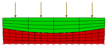
For stress analysis where the interface experiences pure compression, all of the nodes on the interface should deflect the same amount. Thus, choosing Fine bonded to coarse mesh will give more accurate results. See Figure 4.
|
(a) The Model. A simple compression model. |
|
(b) Incorrect. When using Coarse bonded to fine mesh smart bonding, only the nodes on the coarse mesh are forced to follow the displacement of the fine mesh. Thus, the inner nodes on the fine mesh are free to move independently. As seen here in this exaggerated displacement plot, the fine mesh displaces incorrectly. |
|
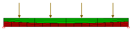
(c) Correct. When using Fine bonded to coarse mesh smart bonding, the nodes on the fine mesh are forced to follow the displacement of the coarse mesh. Both meshes deflect as desired (although the fine mesh is forced to displace linearly at the nodes between the coarse element nodes. This might introduce some inaccuracy). The same exaggerated displacement scale used in (b) is shown here. |
| Figure 4: Stress Analysis Under Pure Compression |
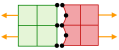
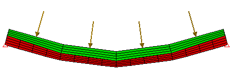
For stress analysis where the interface experiences bending, the nodes on the finer meshed surface must be allowed to move independently of the nodes on the coarser mesh; that is, both sets of nodes should displace so as to create the same radius of curvature. Thus, choosing Coarse bonded to fine mesh will give more accurate results. See Figure 5.
|
(a) The Model. A simple bending model. |
|
(b) Incorrect. When using Fine bonded to coarse mesh smart bonding, the nodes on the fine mesh are forced to follow the displacement of the coarse mesh. By forcing the fine mesh to bend to the same curvature produced by the coarser mesh, the displacement results are less accurate. Because of the kink or sudden change in slope in each set of 4 elements in the bottom part, the stress results in particular would show high stresses. The same exaggerated displacement scale used in (c) is shown here, so this deflection is noticeably smaller. |
|
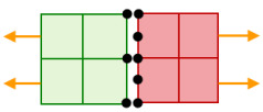
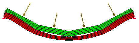
(c) Correct. When using Coarse bonded to fine mesh smart bonding, only the nodes on the coarse mesh are forced to follow the displacement of the fine mesh. Thus, the inner nodes on the fine mesh are free to move independently. Although the displacement of the bottom part may appear to be incorrect because of the separation from the top part (greatly exaggerated here to show the shape better), the fact that both parts follow the proper curvature indicates that these results are more accurate. |
| Figure 5: Stress Analysis Under Pure Bending |
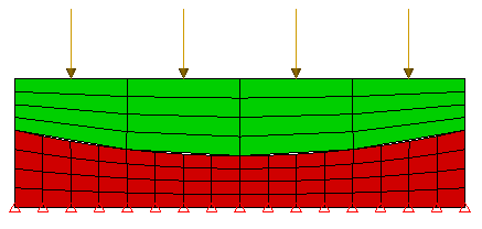
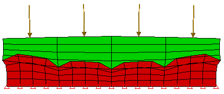
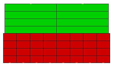
In heat transfer analysis, the flow of heat should be continuous from the finer mesh into the coarser mesh. Thus, choosing Fine bonded to coarse mesh will give more accurate results. See Figure 6. Similar philosophy applies to electrostatic analysis.
|
(a) The Model. A simple two-part model with the bottom surface exposed to a hot environment and the top surface exposed to a cold environment. Since the parts are practically the same width, this 2D model represents a 1-D heat transfer. |
|
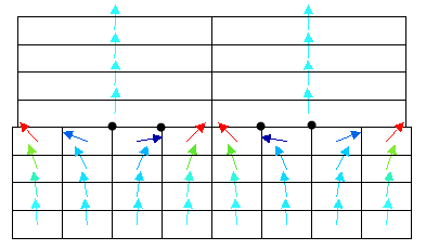
(b) Incorrect. When using Coarse bonded to fine mesh smart bonding, only the nodes on the coarse mesh are forced to follow the temperature of the fine mesh. Thus, the inner nodes on the finer mesh (shown by the dots) are not connected to the top part. These create a blockage to the flow of heat (shown by the arrows at the center of each element.) The heat must flow sideways at the blocked nodes to get to the top part; this creates a less accurate temperature profile. |
|
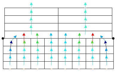
(c) Correct. When using Fine bonded to coarse mesh smart bonding, the nodes on the fine mesh are forced to follow the temperature of the coarse mesh. Thus, only the two outer nodes (shown by the dots) are not connected to the top part. With a reduced blockage to the flow of heat, the heat flux vectors are closer to being parallel (as they should be for 1-D heat transfer). The result is a more accurate temperature profile. |
|
Figure 6: Heat Transfer Analysis |
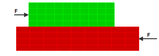
Another consideration in choosing the type of smart bonding is that there needs to be nodes on the chosen surface that physically match the opposite surface. See Figure 7.
|
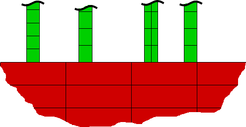
Coarse bonded to fine mesh smart bonding versus Fine bonded to coarse mesh smart bonding. If only nodes on the coarse (bottom, red) part are bonded to the fine (top, green) part by choosing Coarse bonded to fine mesh, then only one node (the one on the right) will be bonded. No other nodes will be bonded since the nodes on the coarse mesh do not touch the other part. If this were a stress analysis, the top part could be statically unstable. For this example to work, the better choice would be Fine bonded to coarse mesh smart bonding. All nodes on the top part will be bonded to the nodes on the bottom part because all of those nodes touch the bottom part. |
| Figure 7: Bonding Drastically Different Mesh Sizes |
Keep in mind that smart bonding approximates the transfer of loads at the boundaries of two parts. In a stress analysis, the continuity of the displacements is conserved. Other quantities such as force, stress, derivative of the displacements are not continuous. Therefore, the results at the boundary where smart bonding occurs may be inaccurate depending on the relative mesh density. However, results remote from the boundary should be accurate, relative to the effects (if any) caused by the smart bonding. If accurate results are desired at the boundary between the parts, smart bonding should not be used; the meshes should be matched instead.
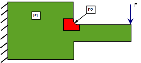
One advantage of smart bonding is to perform what-if studies and change the mesh on one part without the need to re-mesh the entire model. The smart bonding will maintain the connection at the contact faces even though the mesh may not align. See Figure 8.
|
|
Figure 8: Example Use of Smart Bonding. A mesh sensitivity study can be performed by changing the mesh on part 2 [P2] without the need to re-mesh the entire model. The geometry of part 2 can even be changed, such as comparing a chamfer versus a large radius fillet versus a small radius fillet. |
Multipoint Constraint Solution Method
By default, smart bonding uses the Condensation Method to solve your analysis. If you find your analysis doesn't converge or is not performing as you expect, you can try a different
Solution method (see
Multi-Point Constraints). Click
Setup Constraints Multi-Point Constraint and choose from the available
Solution method options.
Constraints Multi-Point Constraint and choose from the available
Solution method options.
If you use the Penalty Method, the accuracy of the solution is controlled by the Penalty multiplier field. A stiffness is applied to the MPC equations, and this stiffness is added to the normal stiffness matrix. The Penalty multiplier, times the maximum diagonal stiffness in the model, is used during the penalty solution. A multiplier of 0 implies that the parts are not connected, and a multiplier of infinity implies a perfect bonding between the parts. Unfortunately, infinite stiffness is not acceptable in a numerical solution, nor is it required. A value in the range of 104 to 106 is recommended. However, some analyses may produce a maximum-to-minimum stiffness warning (max/min stiffness) or fail to find a solution if the penalty multiplier is too large.
To judge the accuracy of the solution, the summary file includes a line with the Satisfaction Factor. A value of 100% indicates that the MPC equations (such as in Figure 1) are satisfied accurately. Any value less than 100% indicates some separation of the parts. It is not possible to say that values below a particular percentage indicate the solution is wrong. Rely on experience to judge when the satisfaction indicates an unacceptable result.
- The solution method you select in the Define Multi-Point Constraints dialog becomes the method used for all features that include MPCs. These features include, but are not limited to, cyclic symmetry, frictionless constraints, smart bonding, and user-defined MPCs. For example, if you want to use the Penalty Method to solve all of your analyses involving smart bonding or other MPC-related features, you can override the default condensation method by selecting Penalty Method in the Define Multi-Point Constraints dialog.
- Smart bonding is applicable to contact between brick, 2D, membrane, and plate elements. Bonded contact involving other element types requires the nodes to match and is not affected by the smart bonding setting.