The slip velocity model described here is used in the wall slip analysis simulation
Experimental observations suggest that the slip velocity depends on the past states of the local wall shear and normal stresses. This slip time-dependency is referred to as retarded slip due to the presence of a relaxation slip time. Most slip velocity models proposed in the literature, however, are continuum static models, where the slip velocity depends on the instantaneous value of the wall shear stress. A modified power-law expression is commonly used:
 [1]
[1]
where:
 is the slip velocity,
 is the wall shear stress,
 is the critical shear stress above which slip occurs,
 is the slip coefficient,
 is the slip exponent.
, the factor
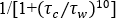 reduces the slip velocity to zero. For shear stress values greater than
, the factor becomes about equal to 1.
reduces the slip velocity to zero. For shear stress values greater than
, the factor becomes about equal to 1.
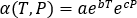
Temperature dependency can be introduced into the slip coefficient by:
 [2]
[2]
where:
 and
and
 are material constants.
Pressure effects on slip velocity can be accounted for either through viscosity modeling, or by including them in the slip coefficient in a similar way to the temperature effects. When the pressure dependency of the viscosity is modeled, the pressure effects on slip velocity are included through the calculation of the wall shear stress. This is the desired method because the effects of pressure on both the onset and slip velocity are included.
If the pressure dependency of the viscosity is not modeled in the melt viscosity, then the slip coefficient defined by equation [2] can be expanded to include the pressure effects on slip velocity:
 [3]
[3]
where:
- ,
, and
 are material constants that need to be characterized.
The empirical power-law slip velocity models are simple algebraic equations relating the slip velocity with shear stress, with temperature and pressure effects modeled in the slip coefficient. The critical shear stress is assumed to be independent of pressure and temperature at the moment.