Use this technical preview to get acquainted with DED settings and performance.
Video length (6:18).
Sample files for use with the tutorials are available on the Download Page.
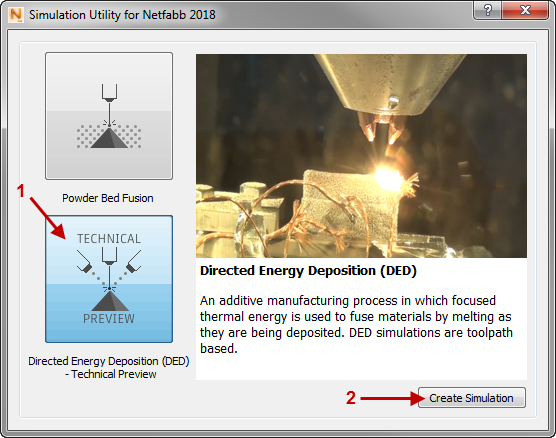
- In Simulation Utility, Click .
- In the dialog that opens, click
Directed Energy Deposition, and then
Create Simulation.
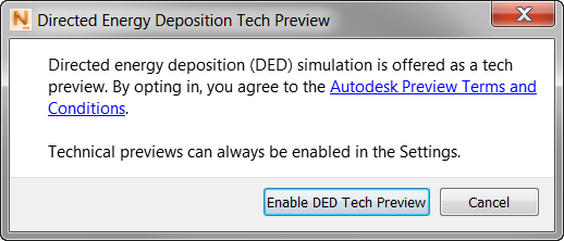
If you have not opted in to the DED technical preview, you will be offered the opportunity to do so.
More information is available at .
-
In the Converted model units dialog, where you are prompted to import a laser vector (LSR) file, click OK.
- Browse to your tutorial example files, and open the file Example_18\path.lsr, and accept the default Converted model units settings.
Let's examine the contents of this file using a text editor.
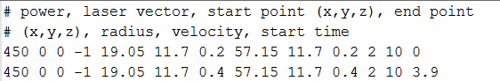
Each laser vector has one line of data, and the order of entries is listed in the top two commented lines:
- First entry on the left is the power, 450 W in this case.
- Laser vector in X Y Z format in relation to the build plate; 0 0 -1 here means that the laser is pointing straight down.
- Starting X Y Z coordinates of the laser pass.
- Ending X Y Z coordinates of the laser pass.
- Laser radius, or half of the bead width in mm.
- Laser velocity in mm/s.
- Start time to activate the path.
- On the Home tab, click Machine to see the Absorption Efficiency setting, typically 30-40% for a laser system. Leave the default value here, and click OK.
- Click
and under
Mechanical Constraints, set
Plate Fixture to
Cantilever.
With this setting, the –X end of the plate is fixed, leaving the other end free to deflect. The other option, Simply Supported, would fix three corners of the build plate in a total of six degrees of freedom.
- Still in the Build Plate dialog, click the
Size tab, and set three
Length values as follows:
- X Length: 60 mm
- Y Length: 10 mm
- Z Length: 5 mm
- Click OK to close the Build Plate dialog.
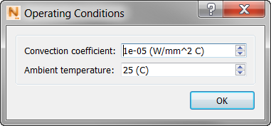
- Click
Operating Conditions, set the
Convection Coefficient to 1e-05, as shown below, and click OK.
- Click
Mesh Settings, and set the values shown below.
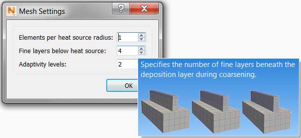
Note that each setting here has an illustrated tooltip:
- Elements per Heat Source Radius controls the mesh density.
- Fine Layers Below Heat Source sets the number of layers that are kept fine, and not adapted below the heat source.
- Adaptivity Levels specifies the maximum number of coarsening generations in the mesh.
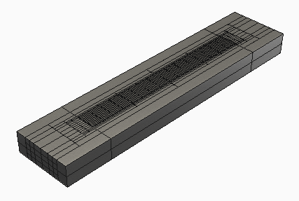
- Click OK to close the Mesh Settings dialog, then click
Mesh Preview and save the project in a suitable location. Load the mesh when it's available, and inspect it.
- Click Solver Settings. Note that here you can set the Analysis Type. Leave it at the default Thermal and Mechanical setting, and click OK.
- Click Solve to start the simulation.
- Load the results when available, and turn on the Temperature results.
- On the Results tab, open
Plot Settings, set the
Displacement Scale to 10 to magnify the displacement results, and click OK.
Play through the results, remembering that the near end of the build plate is fixed. We see the far end of the build plate deflect upwards.
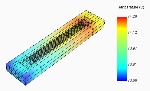
We can follow the deposition passes and see that toward the end, slightly higher temperatures remain in the part, causing the upward deflection of the build plate.
- Turn on Cauchy stress to verify the presence of some stress at the end of the build. On the Results tab, click Plot Settings, and in the dialog, ensure that the
Component value is XX and the
Range is set to Global. Click OK.
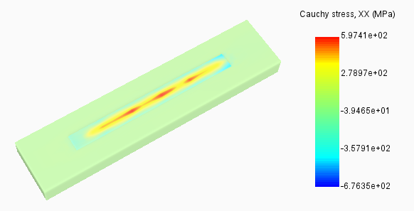
The figure above shows stress levels at the end of the build. For better visibility, element edges were turned off by right-clicking and deselecting Element Edges.